SlideShare a Scribd company logo
Sec on 5.3
    Evalua ng Definite Integrals
           V63.0121.011: Calculus I
         Professor Ma hew Leingang
                New York University


               April 27, 2011


.
Announcements
   Today: 5.3
   Thursday/Friday: Quiz on
   4.1–4.4
   Monday 5/2: 5.4
   Wednesday 5/4: 5.5
   Monday 5/9: Review and
   Movie Day!
   Thursday 5/12: Final
   Exam, 2:00–3:50pm
Objectives
   Use the Evalua on
   Theorem to evaluate
   definite integrals.
   Write an deriva ves as
   indefinite integrals.
   Interpret definite
   integrals as “net change”
   of a func on over an
   interval.
Outline
 Last me: The Definite Integral
     The definite integral as a limit
     Proper es of the integral
 Evalua ng Definite Integrals
    Examples
 The Integral as Net Change
 Indefinite Integrals
    My first table of integrals
 Compu ng Area with integrals
The definite integral as a limit
 Defini on
 If f is a func on defined on [a, b], the definite integral of f from a to
 b is the number
                      ∫ b                ∑n
                          f(x) dx = lim     f(ci ) ∆x
                        a            n→∞
                                           i=1

                 b−a
 where ∆x =          , and for each i, xi = a + i∆x, and ci is a point in
                  n
 [xi−1 , xi ].
The definite integral as a limit

 Theorem
 If f is con nuous on [a, b] or if f has only finitely many jump
 discon nui es, then f is integrable on [a, b]; that is, the definite
            ∫ b
 integral       f(x) dx exists and is the same for any choice of ci .
           a
Notation/Terminology
                            ∫    b
                                     f(x) dx
                             a
   ∫
       — integral sign (swoopy S)
   f(x) — integrand
   a and b — limits of integra on (a is the lower limit and b the
   upper limit)
   dx — ??? (a parenthesis? an infinitesimal? a variable?)
   The process of compu ng an integral is called integra on
Example
          ∫   1
                    4
Es mate                  dx using M4 .
          0       1 + x2
Example
          ∫   1
                    4
Es mate                  dx using M4 .
          0       1 + x2

Solu on
                    1      1      3
We have x0 = 0, x1 = , x2 = , x3 = , x4 = 1.
                    4      2      4
       1       3      5      7
So c1 = , c2 = , c3 = , c4 = .
       8       8      8      8
Example
          ∫   1
                    4
Es mate                  dx using M4 .
          0       1 + x2

Solu on
          (                                                       )
      1            4            4            4            4
 M4 =                  2
                         +          2
                                      +          2
                                                   +
      4       1 + (1/8)    1 + (3/8)    1 + (5/8)    1 + (7/8)2
Example
          ∫   1
                    4
Es mate                  dx using M4 .
          0       1 + x2

Solu on
        (                                           )
      1      4          4          4          4
 M4 =             +          +          +
      4 1 + (1/8)2 1 + (3/8)2 1 + (5/8)2 1 + (7/8)2
        (                            )
      1   4       4       4      4
    =          +     +       +
      4 65/64 73/64 89/64 113/64
Example
          ∫   1
                    4
Es mate                  dx using M4 .
          0       1 + x2

Solu on
        (                                           )
      1      4          4          4          4
 M4 =             +          +          +
      4 1 + (1/8)2 1 + (3/8)2 1 + (5/8)2 1 + (7/8)2
        (                            )
      1    4      4       4      4
    =          +      +       +
      4 65/64 73/64 89/64 113/64
      64 64 64      64
    =    +   +    +    ≈ 3.1468
      65 73 89 113
Properties of the integral
 Theorem (Addi ve Proper es of the Integral)
 Let f and g be integrable func ons on [a, b] and c a constant. Then
       ∫ b
   1.       c dx = c(b − a)
        a
       ∫ b                      ∫ b           ∫ b
   2.       [f(x) + g(x)] dx =      f(x) dx +     g(x) dx.
        a                         a            a
       ∫ b               ∫ b
   3.       cf(x) dx = c     f(x) dx.
       ∫a b               a
                                ∫ b           ∫ b
   4.       [f(x) − g(x)] dx =      f(x) dx −     g(x) dx.
       a                      a            a
More Properties of the Integral
 Conven ons:            ∫                                  ∫
                                a                               b
                                    f(x) dx = −                     f(x) dx
                            b                               a
                                     ∫     a
                                               f(x) dx = 0
                                       a
 This allows us to have
 Theorem
     ∫ c           ∫    b                      ∫     c
  5.     f(x) dx =          f(x) dx +                    f(x) dx for all a, b, and c.
       a            a                            b
Illustrating Property 5
 Theorem
     ∫ c           ∫     b               ∫   c
  5.     f(x) dx =           f(x) dx +           f(x) dx for all a, b, and c.
       a             a                   b


             y


                 .
                         a                                        c   x
                                                 b
Illustrating Property 5
 Theorem
     ∫ c           ∫     b                  ∫     c
  5.     f(x) dx =           f(x) dx +                f(x) dx for all a, b, and c.
       a             a                        b


             y
                              ∫     b
                                        f(x) dx
                                a

                 .
                         a                                             c   x
                                                      b
Illustrating Property 5
 Theorem
     ∫ c           ∫     b                  ∫     c
  5.     f(x) dx =           f(x) dx +                f(x) dx for all a, b, and c.
       a             a                        b


             y
                              ∫     b                     ∫    c
                                        f(x) dx                    f(x) dx
                                a                          b

                 .
                         a                                                   c   x
                                                      b
Illustrating Property 5
 Theorem
     ∫ c           ∫     b                  ∫     c
  5.     f(x) dx =           f(x) dx +                f(x) dx for all a, b, and c.
       a             a                        b


             y
                              ∫     b       ∫ c     ∫ c
                                        f(x) dx f(x) dx f(x) dx
                                a            a             b

                 .
                         a                                             c   x
                                                      b
Illustrating Property 5
 Theorem
     ∫ c           ∫      b               ∫   c
  5.     f(x) dx =            f(x) dx +           f(x) dx for all a, b, and c.
       a              a                   b


             y


                  .
                 a                  c                                  x
                                                                   b
Illustrating Property 5
 Theorem
     ∫ c           ∫      b                 ∫     c
  5.     f(x) dx =            f(x) dx +               f(x) dx for all a, b, and c.
       a              a                       b


             y
                                   ∫    b
                                            f(x) dx
                                    a

                  .
                 a                  c                                      x
                                                                       b
Illustrating Property 5
 Theorem
     ∫ c           ∫      b               ∫   c
  5.     f(x) dx =            f(x) dx +           f(x) dx for all a, b, and c.
       a              a                   b


             y
                                                  ∫   c
                                                     f(x) dx =
                                                   b∫
                                                      b
                                                  −     f(x) dx
                  .                                       c
                 a                  c                                  x
                                                                   b
Illustrating Property 5
 Theorem
     ∫ c           ∫          b               ∫   c
  5.     f(x) dx =                f(x) dx +           f(x) dx for all a, b, and c.
       a                  a                   b


             y
                      ∫                               ∫   c
                          c
                              f(x) dx                    f(x) dx =
                                                       b∫
                      a                                   b
                                                      −     f(x) dx
                  .                                           c
                 a                      c                                  x
                                                                       b
Definite Integrals We Know So Far
  If the integral computes an area
  and we know the area, we can
  use that. For instance,
          ∫ 1√                       y
                            π
                1 − x2 dx =
           0                4
  By brute force we computed             .
   ∫ 1             ∫ 1                       x
        2      1               1
       x dx =          x3 dx =
     0         3     0         4
Comparison Properties of the Integral
 Theorem
 Let f and g be integrable func ons on [a, b].
Comparison Properties of the Integral
 Theorem
 Let f and g be integrable func ons on [a, b].
                                            ∫ b
   6. If f(x) ≥ 0 for all x in [a, b], then     f(x) dx ≥ 0
                                           a
Comparison Properties of the Integral
 Theorem
 Let f and g be integrable func ons on [a, b].
                                            ∫ b
   6. If f(x) ≥ 0 for all x in [a, b], then     f(x) dx ≥ 0
                                             a
                                               ∫ b           ∫   b
   7. If f(x) ≥ g(x) for all x in [a, b], then     f(x) dx ≥         g(x) dx
                                              a              a

  8. If m ≤ f(x) ≤ M for all x in [a, b], then
                                 ∫ b
                  m(b − a) ≤          f(x) dx ≤ M(b − a)
                                     a
Integral of a nonnegative function is nonnegative
  Proof.
  If f(x) ≥ 0 for all x in [a, b], then for
  any number of divisions n and choice
  of sample points {ci }:

          ∑
          n                   ∑
                              n
   Sn =         f(ci ) ∆x ≥         0 · ∆x = 0
          i=1   ≥0            i=1
                                                     .             x
  Since Sn ≥ 0 for all n, the limit of {Sn } is nonnega ve, too:
                        ∫ b
                            f(x) dx = lim Sn ≥ 0
                          a                n→∞
                                                 ≥0
The integral is “increasing”
  Proof.
  Let h(x) = f(x) − g(x). If f(x) ≥ g(x)
  for all x in [a, b], then h(x) ≥ 0 for all                                        f(x)
  x in [a, b]. So by the previous                                        h(x)       g(x)
  property
                ∫ b
                    h(x) dx ≥ 0                               .                       x
                a
  This means that
   ∫ b           ∫      b               ∫   b                        ∫   b
       f(x) dx −            g(x) dx =           (f(x) − g(x)) dx =           h(x) dx ≥ 0
     a              a                   a                            a
Bounding the integral
  Proof.
 If m ≤ f(x) ≤ M on for all x in [a, b], then by
                                                   y
 the previous property
      ∫ b        ∫ b             ∫ b               M
          m dx ≤     f(x) dx ≤        M dx
       a            a             a                                f(x)
 By Property 8, the integral of a constant
 func on is the product of the constant and        m
 the width of the interval. So:
                  ∫ b                                  .             x
     m(b − a) ≤       f(x) dx ≤ M(b − a)                   a   b
                    a
Example
          ∫   2
                  1
Es mate             dx using the comparison proper es.
          1       x
Example
          ∫    2
                   1
Es mate              dx using the comparison proper es.
           1       x

Solu on
Since
                                 1 1 1
                                   ≤ ≤
                                 2  x  1
for all x in [1, 2], we have
                                   ∫    2
                           1                1
                             ·1≤              dx ≤ 1 · 1
                           2        1       x
Ques on
        ∫   2
          1
Es mate     dx with L2 and R2 . Are your es mates overes mates?
        1 x
Underes mates? Impossible to tell?
Ques on
        ∫   2
          1
Es mate     dx with L2 and R2 . Are your es mates overes mates?
        1 x
Underes mates? Impossible to tell?

Answer
Since the integrand is decreasing,
                               ∫ 2
                                   1
                         Rn <        dx < Ln
                                1 x
                   ∫ 2
               7       1      5
for all n. So    <       dx < .
              12    1 x       6
Outline
 Last me: The Definite Integral
     The definite integral as a limit
     Proper es of the integral
 Evalua ng Definite Integrals
    Examples
 The Integral as Net Change
 Indefinite Integrals
    My first table of integrals
 Compu ng Area with integrals
Socratic proof
  The definite integral of velocity
  measures displacement (net
  distance)
  The deriva ve of displacement
  is velocity
  So we can compute
  displacement with the definite
  integral or the an deriva ve of
  velocity
  But any func on can be a
  velocity func on, so . . .
Theorem of the Day
 Theorem (The Second Fundamental Theorem of Calculus)
 Suppose f is integrable on [a, b] and f = F′ for another func on F,
 then                  ∫    b
                                f(x) dx = F(b) − F(a).
                        a
Theorem of the Day
 Theorem (The Second Fundamental Theorem of Calculus)
 Suppose f is integrable on [a, b] and f = F′ for another func on F,
 then                  ∫    b
                                f(x) dx = F(b) − F(a).
                        a


 Note
 In Sec on 5.3, this theorem is called “The Evalua on Theorem”.
 Nobody else in the world calls it that.
Proving the Second FTC
 Proof.
                                                          b−a
     Divide up [a, b] into n pieces of equal width ∆x =       as
                                                           n
     usual.
Proving the Second FTC
 Proof.
                                                               b−a
     Divide up [a, b] into n pieces of equal width ∆x =            as
                                                                n
     usual.
     For each i, F is con nuous on [xi−1 , xi ] and differen able on
     (xi−1 , xi ). So there is a point ci in (xi−1 , xi ) with

                      F(xi ) − F(xi−1 )
                                        = F′ (ci ) = f(ci )
                         xi − xi−1
                        =⇒ f(ci )∆x = F(xi ) − F(xi−1 )
Proving the Second FTC
 Proof.

     Form the Riemann Sum:
Proving the Second FTC
 Proof.

     Form the Riemann Sum:
             ∑
             n                  ∑
                                n
      Sn =         f(ci )∆x =         (F(xi ) − F(xi−1 ))
             i=1                i=1
Proving the Second FTC
 Proof.

     Form the Riemann Sum:
             ∑
             n                  ∑
                                n
      Sn =         f(ci )∆x =         (F(xi ) − F(xi−1 ))
             i=1                i=1
          = (F(x1 ) − F(x0 )) + (F(x2 ) − F(x1 )) + (F(x3 ) − F(x2 )) + · · ·
              · · · + (F(xn−1 ) − F(xn−2 )) + (F(xn ) − F(xn−1 ))
          = F(xn ) − F(x0 ) = F(b) − F(a)
Proving the Second FTC
 Proof.

     We have shown for each n,

                          Sn = F(b) − F(a)

     Which does not depend on n.
Proving the Second FTC
 Proof.

     We have shown for each n,

                           Sn = F(b) − F(a)

     Which does not depend on n.
     So in the limit
         ∫ b
             f(x) dx = lim Sn = lim (F(b) − F(a)) = F(b) − F(a)
          a          n→∞         n→∞
Computing area with the 2nd FTC
 Example
 Find the area between y = x3 and the x-axis, between x = 0 and
 x = 1.


                                               .
Computing area with the 2nd FTC
 Example
 Find the area between y = x3 and the x-axis, between x = 0 and
 x = 1.

 Solu on

        ∫    1               1
                 3      x4           1
   A=            x dx =          =
         0              4    0       4         .
Computing area with the 2nd FTC
 Example
 Find the area between y = x3 and the x-axis, between x = 0 and
 x = 1.

 Solu on

        ∫    1               1
                 3      x4           1
   A=            x dx =          =
         0              4    0       4         .

 Here we use the nota on F(x)|b or [F(x)]b to mean F(b) − F(a).
                              a          a
Computing area with the 2nd FTC
 Example
 Find the area enclosed by the parabola y = x2 and the line y = 1.
Computing area with the 2nd FTC
 Example
 Find the area enclosed by the parabola y = x2 and the line y = 1.


                                                      1

                                                          .
                                              −1                     1
Computing area with the 2nd FTC
 Example
 Find the area enclosed by the parabola y = x2 and the line y = 1.

 Solu on
            ∫   1     [ 3 ]1
                       x
   A=2−    x dx = 2 −
                    2
                                                      1
                       3 −1
        [−1 ( )]
         1      1      4
    =2−    − −       =                                    .
         3      3      3
                                              −1                     1
Computing an integral we
estimated before
 Example
                         ∫   1
                                   4
 Evaluate the integral                  dx.
                         0       1 + x2
Example
          ∫   1
                    4
Es mate                  dx using M4 .
          0       1 + x2

Solu on
        (                                           )
      1      4          4          4          4
 M4 =             +          +          +
      4 1 + (1/8)2 1 + (3/8)2 1 + (5/8)2 1 + (7/8)2
        (                            )
      1    4      4       4      4
    =          +      +       +
      4 65/64 73/64 89/64 113/64
      64 64 64      64
    =    +   +    +    ≈ 3.1468
      65 73 89 113
Computing an integral we
estimated before
 Example
                          ∫    1
                                     4
 Evaluate the integral                    dx.
                           0       1 + x2

 Solu on
     ∫     1                   ∫   1
                 4                       1
                      dx = 4                  dx
       0       1 + x2          0       1 + x2
Computing an integral we
estimated before
 Example
                          ∫    1
                                     4
 Evaluate the integral                    dx.
                           0       1 + x2

 Solu on
     ∫     1                   ∫   1
                 4                       1
                      dx = 4                  dx = 4 arctan(x)|1
                                                               0
       0       1 + x2          0       1 + x2
                        = 4 (arctan 1 − arctan 0)
Computing an integral we
estimated before
 Example
                          ∫    1
                                     4
 Evaluate the integral                    dx.
                           0       1 + x2

 Solu on
     ∫     1                   ∫   1
                 4                1
                      dx = 4            dx = 4 arctan(x)|1
                                                         0
               1 + x2        0 1+x
                                      2
       0                                               (π    )
                        = 4 (arctan 1 − arctan 0) = 4      −0
                                                         4
Computing an integral we
estimated before
 Example
                          ∫    1
                                     4
 Evaluate the integral                    dx.
                           0       1 + x2

 Solu on
     ∫     1                   ∫   1
                 4                1
                      dx = 4            dx = 4 arctan(x)|1
                                                         0
               1 + x2        0 1+x
                                      2
       0                                               (π    )
                        = 4 (arctan 1 − arctan 0) = 4      −0 =π
                                                         4
Computing an integral we
estimated before
 Example
            ∫   2
                    1
 Evaluate             dx.
            1       x
Example
          ∫    2
                   1
Es mate              dx using the comparison proper es.
           1       x

Solu on
Since
                                 1 1 1
                                   ≤ ≤
                                 2  x  1
for all x in [1, 2], we have
                                   ∫    2
                           1                1
                             ·1≤              dx ≤ 1 · 1
                           2        1       x
Computing an integral we
estimated before
 Example
            ∫   2
                    1
 Evaluate             dx.
            1       x

 Solu on
                      ∫     2
                                1
                                  dx
                       1        x
Computing an integral we
estimated before
 Example
            ∫   2
                    1
 Evaluate             dx.
            1       x

 Solu on
                      ∫     2
                                1
                                  dx = ln x|2
                                            1
                       1        x
Computing an integral we
estimated before
 Example
            ∫   2
                    1
 Evaluate             dx.
            1       x

 Solu on
                      ∫     2
                                1
                                  dx = ln x|2 = ln 2 − ln 1
                                            1
                       1        x
Computing an integral we
estimated before
 Example
            ∫   2
                    1
 Evaluate             dx.
            1       x

 Solu on
                      ∫     2
                                1
                                  dx = ln x|2 = ln 2 − ln 1 = ln 2
                                            1
                       1        x
Outline
 Last me: The Definite Integral
     The definite integral as a limit
     Proper es of the integral
 Evalua ng Definite Integrals
    Examples
 The Integral as Net Change
 Indefinite Integrals
    My first table of integrals
 Compu ng Area with integrals
The Integral as Net Change

 Another way to state this theorem is:
                     ∫ b
                         F′ (x) dx = F(b) − F(a),
                       a

 or the integral of a deriva ve along an interval is the net change
 over that interval. This has many interpreta ons.
The Integral as Net Change


 Corollary
 If v(t) represents the velocity of a par cle moving rec linearly, then
                       ∫ t1
                            v(t) dt = s(t1 ) − s(t0 ).
                        t0
The Integral as Net Change


 Corollary
 If MC(x) represents the marginal cost of making x units of a product,
 then                              ∫ x
                     C(x) = C(0) +     MC(q) dq.
                                     0
The Integral as Net Change


 Corollary
 If ρ(x) represents the density of a thin rod at a distance of x from its
 end, then the mass of the rod up to x is
                                    ∫ x
                          m(x) =        ρ(s) ds.
                                     0
Outline
 Last me: The Definite Integral
     The definite integral as a limit
     Proper es of the integral
 Evalua ng Definite Integrals
    Examples
 The Integral as Net Change
 Indefinite Integrals
    My first table of integrals
 Compu ng Area with integrals
A new notation for antiderivatives
 To emphasize the rela onship between an differen a on and
 integra on, we use the indefinite integral nota on
                             ∫
                                f(x) dx

 for any func on whose deriva ve is f(x).
A new notation for antiderivatives
 To emphasize the rela onship between an differen a on and
 integra on, we use the indefinite integral nota on
                             ∫
                                f(x) dx

 for any func on whose deriva ve is f(x). Thus
                        ∫
                           x2 dx = 1 x3 + C.
                                   3
My first table of integrals
 .
  ∫                        ∫           ∫
      [f(x) + g(x)] dx = f(x) dx + g(x) dx
      ∫                                    ∫                 ∫
                    xn+1
         xn dx =         + C (n ̸= −1)         cf(x) dx = c f(x) dx
              ∫ n+1                           ∫
                                                  1
                 ex dx = ex + C                     dx = ln |x| + C
          ∫                                   ∫ x
                                                            ax
             sin x dx = − cos x + C               ax dx =       +C
                                           ∫               ln a
           ∫
               cos x dx = sin x + C           csc2 x dx = − cot x + C
          ∫                              ∫
              sec2 x dx = tan x + C         csc x cot x dx = − csc x + C
        ∫                                ∫
                                                1
           sec x tan x dx = sec x + C       √          dx = arcsin x + C
        ∫                                     1 − x2
               1
                    dx = arctan x + C
            1 + x2
Outline
 Last me: The Definite Integral
     The definite integral as a limit
     Proper es of the integral
 Evalua ng Definite Integrals
    Examples
 The Integral as Net Change
 Indefinite Integrals
    My first table of integrals
 Compu ng Area with integrals
Computing Area with integrals
 Example
 Find the area of the region bounded by the lines x = 1, x = 4, the
 x-axis, and the curve y = ex .
Computing Area with integrals
 Example
 Find the area of the region bounded by the lines x = 1, x = 4, the
 x-axis, and the curve y = ex .

 Solu on
 The answer is        ∫    4
                               ex dx = ex |4 = e4 − e.
                                           1
                       1
Computing Area with integrals
 Example
 Find the area of the region bounded by the curve y = arcsin x, the
 x-axis, and the line x = 1.
Computing Area with integrals
 Example
 Find the area of the region bounded by the curve y = arcsin x, the
 x-axis, and the line x = 1.

 Solu on
                                                     y
                     ∫   1
     The answer is           arcsin x dx, but     π/2
                     0
     we do not know an an deriva ve
     for arcsin.
                                                         .
                                                                  x
                                                              1
Computing Area with integrals
 Example
 Find the area of the region bounded by the curve y = arcsin x, the
 x-axis, and the line x = 1.

 Solu on
                                                     y
     Instead compute the area as                  π/2
         ∫ π/2
     π
       −       sin y dy
     2 0
                                                         .
                                                                  x
                                                              1
Computing Area with integrals
 Example
 Find the area of the region bounded by the curve y = arcsin x, the
 x-axis, and the line x = 1.

 Solu on
                                                     y
     Instead compute the area as                  π/2
         ∫ π/2
     π                   π          π/2
       −       sin y dy = −[− cos x]0
     2 0                 2
                                                         .
                                                                  x
                                                              1
Computing Area with integrals
 Example
 Find the area of the region bounded by the curve y = arcsin x, the
 x-axis, and the line x = 1.

 Solu on
                                                     y
     Instead compute the area as                  π/2
         ∫ π/2
     π                   π          π/2 π
       −       sin y dy = −[− cos x]0 = −1
     2 0                 2              2
                                                         .
                                                                  x
                                                              1
Example
Find the area between the graph of y = (x − 1)(x − 2), the x-axis,
and the ver cal lines x = 0 and x = 3.
Example
Find the area between the graph of y = (x − 1)(x − 2), the x-axis,
and the ver cal lines x = 0 and x = 3.

Solu on
 No ce the func on
 y = (x − 1)(x − 2) is posi ve on [0, 1)      y
 and (2, 3], and nega ve on (1, 2).


                                               .                 x
                                                   1    2    3
Example
Find the area between the graph of y = (x − 1)(x − 2), the x-axis,
and the ver cal lines x = 0 and x = 3.

Solu on
      ∫ 1
  A=      (x2 − 3x + 2) dx                    y
       0
          ∫ 2
       −      (x2 − 3x + 2) dx
           1
                ∫ 3                            .                 x
             +      (x2 − 3x + 2) dx               1    2    3
                 2
Example
Find the area between the graph of y = (x − 1)(x − 2), the x-axis,
and the ver cal lines x = 0 and x = 3.

Solu on
      ∫ 1
  A=      (x − 1)(x − 2) dx                   y
       0
          ∫ 2
       −      (x − 1)(x − 2) dx
           1
               ∫ 3                             .                 x
             +     (x − 1)(x − 2) dx               1    2    3
                2
Example
Find the area between the graph of y = (x − 1)(x − 2), the x-axis,
and the ver cal lines x = 0 and x = 3.

Solu on

       [1               ]1                    y
  A=    3 x − 3 x2 + 2x 0
            3
                2
            [1 3 3 2           ]2
          − 3x − 2x +        2x 1
            [                  ]3
          + 1 x3 − 3 x2 +
              3     2        2x 2              .                 x
                                      11           1    2    3
                                    =
                                       6
Interpretation of “negative area”
in motion

 There is an analog in rectlinear mo on:
     ∫ t1
           v(t) dt is net distance traveled.
       t0
     ∫ t1
           |v(t)| dt is total distance traveled.
       t0
What about the constant?
   It seems we forgot about the +C when we say for instance
                   ∫ 1            1
                               x4    1       1
                        3
                       x dx =       = −0=
                    0          4 0 4         4
   But no ce
        [ 4   ]1 (      )
         x         1                1          1
            +C =     + C − (0 + C) = + C − C =
          4    0   4                4          4
   no ma er what C is.
   So in an differen a on for definite integrals, the constant is
   immaterial.
Summary
  The second Fundamental Theorem of Calculus:
                   ∫ b
                       f(x) dx = F(b) − F(a)
                      a

  where F′ = f.
  Definite integrals represent net change of a func on over an
  interval.                                      ∫
  We write an deriva ves as indefinite integrals f(x) dx

More Related Content

What's hot (20)

PPTX
Maxima and minima
Umesh Pandey
 
PDF
Ideals and factor rings
dianageorge27
 
PPT
Limits
admercano101
 
PDF
The Definite Integral
Silvius
 
PPTX
Integral calculus
IndiraDevi24
 
PPTX
First order linear differential equation
Nofal Umair
 
PPTX
Types of function
SanaullahMemon10
 
PPT
Function transformations
Terry Gastauer
 
PPT
systems of linear equations & matrices
Student
 
PPT
THE BINOMIAL THEOREM
τυσηαρ ηαβιβ
 
PPT
L19 increasing &amp; decreasing functions
James Tagara
 
PPTX
Double Integrals
kishor pokar
 
PDF
Lesson 27: Integration by Substitution (slides)
Matthew Leingang
 
PPT
functions limits and continuity
Pume Ananda
 
PPTX
Gaussian Elimination Method
Andi Firdaus
 
PPTX
Exponential and logarithmic functions
Njabulo Nkabinde
 
PDF
Lesson 11: Limits and Continuity
Matthew Leingang
 
PPTX
APPLICATION OF PARTIAL DIFFERENTIATION
Dhrupal Patel
 
PPTX
Limit of functions
Juan Apolinario Reyes
 
Maxima and minima
Umesh Pandey
 
Ideals and factor rings
dianageorge27
 
Limits
admercano101
 
The Definite Integral
Silvius
 
Integral calculus
IndiraDevi24
 
First order linear differential equation
Nofal Umair
 
Types of function
SanaullahMemon10
 
Function transformations
Terry Gastauer
 
systems of linear equations & matrices
Student
 
THE BINOMIAL THEOREM
τυσηαρ ηαβιβ
 
L19 increasing &amp; decreasing functions
James Tagara
 
Double Integrals
kishor pokar
 
Lesson 27: Integration by Substitution (slides)
Matthew Leingang
 
functions limits and continuity
Pume Ananda
 
Gaussian Elimination Method
Andi Firdaus
 
Exponential and logarithmic functions
Njabulo Nkabinde
 
Lesson 11: Limits and Continuity
Matthew Leingang
 
APPLICATION OF PARTIAL DIFFERENTIATION
Dhrupal Patel
 
Limit of functions
Juan Apolinario Reyes
 

Viewers also liked (20)

PPTX
Definite Integral Review
Sharon Henry
 
PPTX
Lesson 8 the definite integrals
Lawrence De Vera
 
PPTX
Lesson 9 transcendental functions
Lawrence De Vera
 
PPTX
Lesson 10 techniques of integration
Lawrence De Vera
 
PDF
Lesson 23: Antiderivatives (slides)
Matthew Leingang
 
PDF
Lesson 22: Optimization Problems (slides)
Matthew Leingang
 
PPT
Introduction
Matthew Leingang
 
PDF
Lesson 6: The Derivative
Matthew Leingang
 
PDF
Lesson 9: The Product and Quotient Rules
Matthew Leingang
 
PDF
Lesson 4: Continuity
Matthew Leingang
 
PDF
Lesson 5: Limits Involving Infinity
Matthew Leingang
 
PDF
Lesson 8: Basic Differentiation Rules
Matthew Leingang
 
PDF
Lesson 7: The Derivative as a Function
Matthew Leingang
 
PDF
Lesson 2: The Concept of Limit
Matthew Leingang
 
PDF
Lesson 24: Areas and Distances, The Definite Integral (slides)
Matthew Leingang
 
PDF
Lesson 12: Linear Approximation
Matthew Leingang
 
PDF
Lesson 21: Curve Sketching
Matthew Leingang
 
PDF
Lesson 1: Functions
Matthew Leingang
 
PDF
Lesson22 -optimization_problems_slides
Matthew Leingang
 
PDF
Lesson 3: Limit Laws
Matthew Leingang
 
Definite Integral Review
Sharon Henry
 
Lesson 8 the definite integrals
Lawrence De Vera
 
Lesson 9 transcendental functions
Lawrence De Vera
 
Lesson 10 techniques of integration
Lawrence De Vera
 
Lesson 23: Antiderivatives (slides)
Matthew Leingang
 
Lesson 22: Optimization Problems (slides)
Matthew Leingang
 
Introduction
Matthew Leingang
 
Lesson 6: The Derivative
Matthew Leingang
 
Lesson 9: The Product and Quotient Rules
Matthew Leingang
 
Lesson 4: Continuity
Matthew Leingang
 
Lesson 5: Limits Involving Infinity
Matthew Leingang
 
Lesson 8: Basic Differentiation Rules
Matthew Leingang
 
Lesson 7: The Derivative as a Function
Matthew Leingang
 
Lesson 2: The Concept of Limit
Matthew Leingang
 
Lesson 24: Areas and Distances, The Definite Integral (slides)
Matthew Leingang
 
Lesson 12: Linear Approximation
Matthew Leingang
 
Lesson 21: Curve Sketching
Matthew Leingang
 
Lesson 1: Functions
Matthew Leingang
 
Lesson22 -optimization_problems_slides
Matthew Leingang
 
Lesson 3: Limit Laws
Matthew Leingang
 
Ad

Similar to Lesson 25: Evaluating Definite Integrals (slides) (20)

PDF
Lesson 27: Evaluating Definite Integrals
Matthew Leingang
 
PDF
Lesson 27: Evaluating Definite Integrals
Matthew Leingang
 
PDF
Lesson 25: Evaluating Definite Integrals (Section 10 version)
Matthew Leingang
 
PDF
Lesson 25: Evaluating Definite Integrals (Section 4 version)
Matthew Leingang
 
PDF
Lesson 28: The Fundamental Theorem of Calculus
Matthew Leingang
 
PDF
Lesson 28: The Fundamental Theorem of Calculus
Matthew Leingang
 
PDF
Lesson 30: The Definite Integral
Matthew Leingang
 
PDF
Lesson 26: The Fundamental Theorem of Calculus (slides)
Matthew Leingang
 
PDF
Lesson 26: The Fundamental Theorem of Calculus (slides)
Matthew Leingang
 
PDF
Lesson 26: The Fundamental Theorem of Calculus (slides)
Mel Anthony Pepito
 
PDF
Lesson 25: Evaluating Definite Integrals (Section 041 slides)
Matthew Leingang
 
PDF
Lesson 25: Evaluating Definite Integrals (Section 041 slides)
Mel Anthony Pepito
 
PDF
Lesson 26: The Fundamental Theorem of Calculus (Section 10 version)
Matthew Leingang
 
PDF
Lesson 31: Evaluating Definite Integrals
Matthew Leingang
 
PDF
Lesson 29: Integration by Substition
Matthew Leingang
 
PDF
Lesson 29: Integration by Substition (worksheet solutions)
Matthew Leingang
 
PDF
Final Exam Review (Integration)
Matthew Leingang
 
PDF
Business math
sanjida_yeasmin
 
PDF
Lesson 26: The Fundamental Theorem of Calculus (Section 4 version)
Matthew Leingang
 
PDF
Evaluating definite integrals
منتدى الرياضيات المتقدمة
 
Lesson 27: Evaluating Definite Integrals
Matthew Leingang
 
Lesson 27: Evaluating Definite Integrals
Matthew Leingang
 
Lesson 25: Evaluating Definite Integrals (Section 10 version)
Matthew Leingang
 
Lesson 25: Evaluating Definite Integrals (Section 4 version)
Matthew Leingang
 
Lesson 28: The Fundamental Theorem of Calculus
Matthew Leingang
 
Lesson 28: The Fundamental Theorem of Calculus
Matthew Leingang
 
Lesson 30: The Definite Integral
Matthew Leingang
 
Lesson 26: The Fundamental Theorem of Calculus (slides)
Matthew Leingang
 
Lesson 26: The Fundamental Theorem of Calculus (slides)
Matthew Leingang
 
Lesson 26: The Fundamental Theorem of Calculus (slides)
Mel Anthony Pepito
 
Lesson 25: Evaluating Definite Integrals (Section 041 slides)
Matthew Leingang
 
Lesson 25: Evaluating Definite Integrals (Section 041 slides)
Mel Anthony Pepito
 
Lesson 26: The Fundamental Theorem of Calculus (Section 10 version)
Matthew Leingang
 
Lesson 31: Evaluating Definite Integrals
Matthew Leingang
 
Lesson 29: Integration by Substition
Matthew Leingang
 
Lesson 29: Integration by Substition (worksheet solutions)
Matthew Leingang
 
Final Exam Review (Integration)
Matthew Leingang
 
Business math
sanjida_yeasmin
 
Lesson 26: The Fundamental Theorem of Calculus (Section 4 version)
Matthew Leingang
 
Evaluating definite integrals
منتدى الرياضيات المتقدمة
 
Ad

More from Matthew Leingang (20)

PPT
Making Lesson Plans
Matthew Leingang
 
PPT
Streamlining assessment, feedback, and archival with auto-multiple-choice
Matthew Leingang
 
PDF
Electronic Grading of Paper Assessments
Matthew Leingang
 
PDF
Lesson 27: Integration by Substitution (handout)
Matthew Leingang
 
PDF
Lesson 26: The Fundamental Theorem of Calculus (handout)
Matthew Leingang
 
PDF
Lesson 25: Evaluating Definite Integrals (handout)
Matthew Leingang
 
PDF
Lesson 24: Areas and Distances, The Definite Integral (handout)
Matthew Leingang
 
PDF
Lesson 23: Antiderivatives (slides)
Matthew Leingang
 
PDF
Lesson 22: Optimization Problems (handout)
Matthew Leingang
 
PDF
Lesson 21: Curve Sketching (slides)
Matthew Leingang
 
PDF
Lesson 21: Curve Sketching (handout)
Matthew Leingang
 
PDF
Lesson 20: Derivatives and the Shapes of Curves (slides)
Matthew Leingang
 
PDF
Lesson 20: Derivatives and the Shapes of Curves (handout)
Matthew Leingang
 
PDF
Lesson 19: The Mean Value Theorem (slides)
Matthew Leingang
 
PDF
Lesson 18: Maximum and Minimum Values (slides)
Matthew Leingang
 
PDF
Lesson 17: Indeterminate forms and l'Hôpital's Rule (slides)
Matthew Leingang
 
PDF
Lesson 18: Maximum and Minimum Values (handout)
Matthew Leingang
 
PDF
Lesson 17: Indeterminate forms and l'Hôpital's Rule (handout)
Matthew Leingang
 
PDF
Lesson 16: Inverse Trigonometric Functions (slides)
Matthew Leingang
 
PDF
Lesson 16: Inverse Trigonometric Functions (handout)
Matthew Leingang
 
Making Lesson Plans
Matthew Leingang
 
Streamlining assessment, feedback, and archival with auto-multiple-choice
Matthew Leingang
 
Electronic Grading of Paper Assessments
Matthew Leingang
 
Lesson 27: Integration by Substitution (handout)
Matthew Leingang
 
Lesson 26: The Fundamental Theorem of Calculus (handout)
Matthew Leingang
 
Lesson 25: Evaluating Definite Integrals (handout)
Matthew Leingang
 
Lesson 24: Areas and Distances, The Definite Integral (handout)
Matthew Leingang
 
Lesson 23: Antiderivatives (slides)
Matthew Leingang
 
Lesson 22: Optimization Problems (handout)
Matthew Leingang
 
Lesson 21: Curve Sketching (slides)
Matthew Leingang
 
Lesson 21: Curve Sketching (handout)
Matthew Leingang
 
Lesson 20: Derivatives and the Shapes of Curves (slides)
Matthew Leingang
 
Lesson 20: Derivatives and the Shapes of Curves (handout)
Matthew Leingang
 
Lesson 19: The Mean Value Theorem (slides)
Matthew Leingang
 
Lesson 18: Maximum and Minimum Values (slides)
Matthew Leingang
 
Lesson 17: Indeterminate forms and l'Hôpital's Rule (slides)
Matthew Leingang
 
Lesson 18: Maximum and Minimum Values (handout)
Matthew Leingang
 
Lesson 17: Indeterminate forms and l'Hôpital's Rule (handout)
Matthew Leingang
 
Lesson 16: Inverse Trigonometric Functions (slides)
Matthew Leingang
 
Lesson 16: Inverse Trigonometric Functions (handout)
Matthew Leingang
 

Recently uploaded (20)

PDF
Meetup Kickoff & Welcome - Rohit Yadav, CSIUG Chairman
ShapeBlue
 
PDF
Human-centred design in online workplace learning and relationship to engagem...
Tracy Tang
 
PDF
Fl Studio 24.2.2 Build 4597 Crack for Windows Free Download 2025
faizk77g
 
PDF
Windsurf Meetup Ottawa 2025-07-12 - Planning Mode at Reliza.pdf
Pavel Shukhman
 
PDF
Rethinking Security Operations - SOC Evolution Journey.pdf
Haris Chughtai
 
PDF
Building Resilience with Digital Twins : Lessons from Korea
SANGHEE SHIN
 
PPTX
Building a Production-Ready Barts Health Secure Data Environment Tooling, Acc...
Barts Health
 
PDF
SWEBOK Guide and Software Services Engineering Education
Hironori Washizaki
 
PDF
Predicting the unpredictable: re-engineering recommendation algorithms for fr...
Speck&Tech
 
PDF
CIFDAQ Weekly Market Wrap for 11th July 2025
CIFDAQ
 
PDF
LLMs.txt: Easily Control How AI Crawls Your Site
Keploy
 
PPTX
Top Managed Service Providers in Los Angeles
Captain IT
 
PDF
Empower Inclusion Through Accessible Java Applications
Ana-Maria Mihalceanu
 
PDF
July Patch Tuesday
Ivanti
 
PDF
Women in Automation Presents: Reinventing Yourself — Bold Career Pivots That ...
DianaGray10
 
PDF
Apache CloudStack 201: Let's Design & Build an IaaS Cloud
ShapeBlue
 
PDF
Why Orbit Edge Tech is a Top Next JS Development Company in 2025
mahendraalaska08
 
PDF
Français Patch Tuesday - Juillet
Ivanti
 
PDF
CloudStack GPU Integration - Rohit Yadav
ShapeBlue
 
PDF
HCIP-Data Center Facility Deployment V2.0 Training Material (Without Remarks ...
mcastillo49
 
Meetup Kickoff & Welcome - Rohit Yadav, CSIUG Chairman
ShapeBlue
 
Human-centred design in online workplace learning and relationship to engagem...
Tracy Tang
 
Fl Studio 24.2.2 Build 4597 Crack for Windows Free Download 2025
faizk77g
 
Windsurf Meetup Ottawa 2025-07-12 - Planning Mode at Reliza.pdf
Pavel Shukhman
 
Rethinking Security Operations - SOC Evolution Journey.pdf
Haris Chughtai
 
Building Resilience with Digital Twins : Lessons from Korea
SANGHEE SHIN
 
Building a Production-Ready Barts Health Secure Data Environment Tooling, Acc...
Barts Health
 
SWEBOK Guide and Software Services Engineering Education
Hironori Washizaki
 
Predicting the unpredictable: re-engineering recommendation algorithms for fr...
Speck&Tech
 
CIFDAQ Weekly Market Wrap for 11th July 2025
CIFDAQ
 
LLMs.txt: Easily Control How AI Crawls Your Site
Keploy
 
Top Managed Service Providers in Los Angeles
Captain IT
 
Empower Inclusion Through Accessible Java Applications
Ana-Maria Mihalceanu
 
July Patch Tuesday
Ivanti
 
Women in Automation Presents: Reinventing Yourself — Bold Career Pivots That ...
DianaGray10
 
Apache CloudStack 201: Let's Design & Build an IaaS Cloud
ShapeBlue
 
Why Orbit Edge Tech is a Top Next JS Development Company in 2025
mahendraalaska08
 
Français Patch Tuesday - Juillet
Ivanti
 
CloudStack GPU Integration - Rohit Yadav
ShapeBlue
 
HCIP-Data Center Facility Deployment V2.0 Training Material (Without Remarks ...
mcastillo49
 

Lesson 25: Evaluating Definite Integrals (slides)

  • 1. Sec on 5.3 Evalua ng Definite Integrals V63.0121.011: Calculus I Professor Ma hew Leingang New York University April 27, 2011 .
  • 2. Announcements Today: 5.3 Thursday/Friday: Quiz on 4.1–4.4 Monday 5/2: 5.4 Wednesday 5/4: 5.5 Monday 5/9: Review and Movie Day! Thursday 5/12: Final Exam, 2:00–3:50pm
  • 3. Objectives Use the Evalua on Theorem to evaluate definite integrals. Write an deriva ves as indefinite integrals. Interpret definite integrals as “net change” of a func on over an interval.
  • 4. Outline Last me: The Definite Integral The definite integral as a limit Proper es of the integral Evalua ng Definite Integrals Examples The Integral as Net Change Indefinite Integrals My first table of integrals Compu ng Area with integrals
  • 5. The definite integral as a limit Defini on If f is a func on defined on [a, b], the definite integral of f from a to b is the number ∫ b ∑n f(x) dx = lim f(ci ) ∆x a n→∞ i=1 b−a where ∆x = , and for each i, xi = a + i∆x, and ci is a point in n [xi−1 , xi ].
  • 6. The definite integral as a limit Theorem If f is con nuous on [a, b] or if f has only finitely many jump discon nui es, then f is integrable on [a, b]; that is, the definite ∫ b integral f(x) dx exists and is the same for any choice of ci . a
  • 7. Notation/Terminology ∫ b f(x) dx a ∫ — integral sign (swoopy S) f(x) — integrand a and b — limits of integra on (a is the lower limit and b the upper limit) dx — ??? (a parenthesis? an infinitesimal? a variable?) The process of compu ng an integral is called integra on
  • 8. Example ∫ 1 4 Es mate dx using M4 . 0 1 + x2
  • 9. Example ∫ 1 4 Es mate dx using M4 . 0 1 + x2 Solu on 1 1 3 We have x0 = 0, x1 = , x2 = , x3 = , x4 = 1. 4 2 4 1 3 5 7 So c1 = , c2 = , c3 = , c4 = . 8 8 8 8
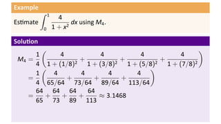
  • 10. Example ∫ 1 4 Es mate dx using M4 . 0 1 + x2 Solu on ( ) 1 4 4 4 4 M4 = 2 + 2 + 2 + 4 1 + (1/8) 1 + (3/8) 1 + (5/8) 1 + (7/8)2
  • 11. Example ∫ 1 4 Es mate dx using M4 . 0 1 + x2 Solu on ( ) 1 4 4 4 4 M4 = + + + 4 1 + (1/8)2 1 + (3/8)2 1 + (5/8)2 1 + (7/8)2 ( ) 1 4 4 4 4 = + + + 4 65/64 73/64 89/64 113/64
  • 12. Example ∫ 1 4 Es mate dx using M4 . 0 1 + x2 Solu on ( ) 1 4 4 4 4 M4 = + + + 4 1 + (1/8)2 1 + (3/8)2 1 + (5/8)2 1 + (7/8)2 ( ) 1 4 4 4 4 = + + + 4 65/64 73/64 89/64 113/64 64 64 64 64 = + + + ≈ 3.1468 65 73 89 113
  • 13. Properties of the integral Theorem (Addi ve Proper es of the Integral) Let f and g be integrable func ons on [a, b] and c a constant. Then ∫ b 1. c dx = c(b − a) a ∫ b ∫ b ∫ b 2. [f(x) + g(x)] dx = f(x) dx + g(x) dx. a a a ∫ b ∫ b 3. cf(x) dx = c f(x) dx. ∫a b a ∫ b ∫ b 4. [f(x) − g(x)] dx = f(x) dx − g(x) dx. a a a
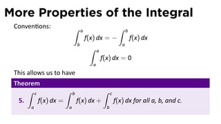
  • 14. More Properties of the Integral Conven ons: ∫ ∫ a b f(x) dx = − f(x) dx b a ∫ a f(x) dx = 0 a This allows us to have Theorem ∫ c ∫ b ∫ c 5. f(x) dx = f(x) dx + f(x) dx for all a, b, and c. a a b
  • 15. Illustrating Property 5 Theorem ∫ c ∫ b ∫ c 5. f(x) dx = f(x) dx + f(x) dx for all a, b, and c. a a b y . a c x b
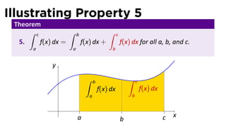
  • 16. Illustrating Property 5 Theorem ∫ c ∫ b ∫ c 5. f(x) dx = f(x) dx + f(x) dx for all a, b, and c. a a b y ∫ b f(x) dx a . a c x b
  • 17. Illustrating Property 5 Theorem ∫ c ∫ b ∫ c 5. f(x) dx = f(x) dx + f(x) dx for all a, b, and c. a a b y ∫ b ∫ c f(x) dx f(x) dx a b . a c x b
  • 18. Illustrating Property 5 Theorem ∫ c ∫ b ∫ c 5. f(x) dx = f(x) dx + f(x) dx for all a, b, and c. a a b y ∫ b ∫ c ∫ c f(x) dx f(x) dx f(x) dx a a b . a c x b
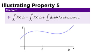
  • 19. Illustrating Property 5 Theorem ∫ c ∫ b ∫ c 5. f(x) dx = f(x) dx + f(x) dx for all a, b, and c. a a b y . a c x b
  • 20. Illustrating Property 5 Theorem ∫ c ∫ b ∫ c 5. f(x) dx = f(x) dx + f(x) dx for all a, b, and c. a a b y ∫ b f(x) dx a . a c x b
  • 21. Illustrating Property 5 Theorem ∫ c ∫ b ∫ c 5. f(x) dx = f(x) dx + f(x) dx for all a, b, and c. a a b y ∫ c f(x) dx = b∫ b − f(x) dx . c a c x b
  • 22. Illustrating Property 5 Theorem ∫ c ∫ b ∫ c 5. f(x) dx = f(x) dx + f(x) dx for all a, b, and c. a a b y ∫ ∫ c c f(x) dx f(x) dx = b∫ a b − f(x) dx . c a c x b
  • 23. Definite Integrals We Know So Far If the integral computes an area and we know the area, we can use that. For instance, ∫ 1√ y π 1 − x2 dx = 0 4 By brute force we computed . ∫ 1 ∫ 1 x 2 1 1 x dx = x3 dx = 0 3 0 4
  • 24. Comparison Properties of the Integral Theorem Let f and g be integrable func ons on [a, b].
  • 25. Comparison Properties of the Integral Theorem Let f and g be integrable func ons on [a, b]. ∫ b 6. If f(x) ≥ 0 for all x in [a, b], then f(x) dx ≥ 0 a
  • 26. Comparison Properties of the Integral Theorem Let f and g be integrable func ons on [a, b]. ∫ b 6. If f(x) ≥ 0 for all x in [a, b], then f(x) dx ≥ 0 a ∫ b ∫ b 7. If f(x) ≥ g(x) for all x in [a, b], then f(x) dx ≥ g(x) dx a a
  • 27. Comparison Properties of the Integral Theorem Let f and g be integrable func ons on [a, b]. ∫ b 6. If f(x) ≥ 0 for all x in [a, b], then f(x) dx ≥ 0 a ∫ b ∫ b 7. If f(x) ≥ g(x) for all x in [a, b], then f(x) dx ≥ g(x) dx a a 8. If m ≤ f(x) ≤ M for all x in [a, b], then ∫ b m(b − a) ≤ f(x) dx ≤ M(b − a) a
  • 28. Integral of a nonnegative function is nonnegative Proof. If f(x) ≥ 0 for all x in [a, b], then for any number of divisions n and choice of sample points {ci }: ∑ n ∑ n Sn = f(ci ) ∆x ≥ 0 · ∆x = 0 i=1 ≥0 i=1 . x Since Sn ≥ 0 for all n, the limit of {Sn } is nonnega ve, too: ∫ b f(x) dx = lim Sn ≥ 0 a n→∞ ≥0
  • 29. The integral is “increasing” Proof. Let h(x) = f(x) − g(x). If f(x) ≥ g(x) for all x in [a, b], then h(x) ≥ 0 for all f(x) x in [a, b]. So by the previous h(x) g(x) property ∫ b h(x) dx ≥ 0 . x a This means that ∫ b ∫ b ∫ b ∫ b f(x) dx − g(x) dx = (f(x) − g(x)) dx = h(x) dx ≥ 0 a a a a
  • 30. Bounding the integral Proof. If m ≤ f(x) ≤ M on for all x in [a, b], then by y the previous property ∫ b ∫ b ∫ b M m dx ≤ f(x) dx ≤ M dx a a a f(x) By Property 8, the integral of a constant func on is the product of the constant and m the width of the interval. So: ∫ b . x m(b − a) ≤ f(x) dx ≤ M(b − a) a b a
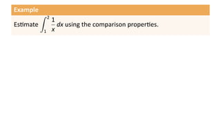
  • 31. Example ∫ 2 1 Es mate dx using the comparison proper es. 1 x
  • 32. Example ∫ 2 1 Es mate dx using the comparison proper es. 1 x Solu on Since 1 1 1 ≤ ≤ 2 x 1 for all x in [1, 2], we have ∫ 2 1 1 ·1≤ dx ≤ 1 · 1 2 1 x
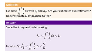
  • 33. Ques on ∫ 2 1 Es mate dx with L2 and R2 . Are your es mates overes mates? 1 x Underes mates? Impossible to tell?
  • 34. Ques on ∫ 2 1 Es mate dx with L2 and R2 . Are your es mates overes mates? 1 x Underes mates? Impossible to tell? Answer Since the integrand is decreasing, ∫ 2 1 Rn < dx < Ln 1 x ∫ 2 7 1 5 for all n. So < dx < . 12 1 x 6
  • 35. Outline Last me: The Definite Integral The definite integral as a limit Proper es of the integral Evalua ng Definite Integrals Examples The Integral as Net Change Indefinite Integrals My first table of integrals Compu ng Area with integrals
  • 36. Socratic proof The definite integral of velocity measures displacement (net distance) The deriva ve of displacement is velocity So we can compute displacement with the definite integral or the an deriva ve of velocity But any func on can be a velocity func on, so . . .
  • 37. Theorem of the Day Theorem (The Second Fundamental Theorem of Calculus) Suppose f is integrable on [a, b] and f = F′ for another func on F, then ∫ b f(x) dx = F(b) − F(a). a
  • 38. Theorem of the Day Theorem (The Second Fundamental Theorem of Calculus) Suppose f is integrable on [a, b] and f = F′ for another func on F, then ∫ b f(x) dx = F(b) − F(a). a Note In Sec on 5.3, this theorem is called “The Evalua on Theorem”. Nobody else in the world calls it that.
  • 39. Proving the Second FTC Proof. b−a Divide up [a, b] into n pieces of equal width ∆x = as n usual.
  • 40. Proving the Second FTC Proof. b−a Divide up [a, b] into n pieces of equal width ∆x = as n usual. For each i, F is con nuous on [xi−1 , xi ] and differen able on (xi−1 , xi ). So there is a point ci in (xi−1 , xi ) with F(xi ) − F(xi−1 ) = F′ (ci ) = f(ci ) xi − xi−1
  • 41. Proving the Second FTC Proof. b−a Divide up [a, b] into n pieces of equal width ∆x = as n usual. For each i, F is con nuous on [xi−1 , xi ] and differen able on (xi−1 , xi ). So there is a point ci in (xi−1 , xi ) with F(xi ) − F(xi−1 ) = F′ (ci ) = f(ci ) xi − xi−1 =⇒ f(ci )∆x = F(xi ) − F(xi−1 )
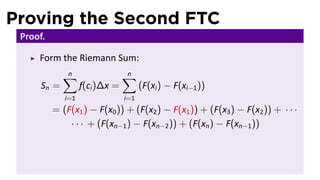
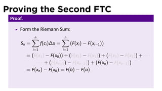
  • 42. Proving the Second FTC Proof. Form the Riemann Sum:
  • 43. Proving the Second FTC Proof. Form the Riemann Sum: ∑ n ∑ n Sn = f(ci )∆x = (F(xi ) − F(xi−1 )) i=1 i=1
  • 44. Proving the Second FTC Proof. Form the Riemann Sum: ∑ n ∑ n Sn = f(ci )∆x = (F(xi ) − F(xi−1 )) i=1 i=1 = (F(x1 ) − F(x0 )) + (F(x2 ) − F(x1 )) + (F(x3 ) − F(x2 )) + · · · · · · + (F(xn−1 ) − F(xn−2 )) + (F(xn ) − F(xn−1 ))
  • 45. Proving the Second FTC Proof. Form the Riemann Sum: ∑ n ∑ n Sn = f(ci )∆x = (F(xi ) − F(xi−1 )) i=1 i=1 = (F(x1 ) − F(x0 )) + (F(x2 ) − F(x1 )) + (F(x3 ) − F(x2 )) + · · · · · · + (F(xn−1 ) − F(xn−2 )) + (F(xn ) − F(xn−1 ))
  • 46. Proving the Second FTC Proof. Form the Riemann Sum: ∑ n ∑ n Sn = f(ci )∆x = (F(xi ) − F(xi−1 )) i=1 i=1 = (F(x1 ) − F(x0 )) + (F(x2 ) − F(x1 )) + (F(x3 ) − F(x2 )) + · · · · · · + (F(xn−1 ) − F(xn−2 )) + (F(xn ) − F(xn−1 ))
  • 47. Proving the Second FTC Proof. Form the Riemann Sum: ∑ n ∑ n Sn = f(ci )∆x = (F(xi ) − F(xi−1 )) i=1 i=1 = (F(x1 ) − F(x0 )) + (F(x2 ) − F(x1 )) + (F(x3 ) − F(x2 )) + · · · · · · + (F(xn−1 ) − F(xn−2 )) + (F(xn ) − F(xn−1 ))
  • 48. Proving the Second FTC Proof. Form the Riemann Sum: ∑ n ∑ n Sn = f(ci )∆x = (F(xi ) − F(xi−1 )) i=1 i=1 = (F(x1 ) − F(x0 )) + (F(x2 ) − F(x1 )) + (F(x3 ) − F(x2 )) + · · · · · · + (F(xn−1 ) − F(xn−2 )) + (F(xn ) − F(xn−1 ))
  • 49. Proving the Second FTC Proof. Form the Riemann Sum: ∑ n ∑ n Sn = f(ci )∆x = (F(xi ) − F(xi−1 )) i=1 i=1 = (F(x1 ) − F(x0 )) + (F(x2 ) − F(x1 )) + (F(x3 ) − F(x2 )) + · · · · · · + (F(xn−1 ) − F(xn−2 )) + (F(xn ) − F(xn−1 ))
  • 50. Proving the Second FTC Proof. Form the Riemann Sum: ∑ n ∑ n Sn = f(ci )∆x = (F(xi ) − F(xi−1 )) i=1 i=1 = (F(x1 ) − F(x0 )) + (F(x2 ) − F(x1 )) + (F(x3 ) − F(x2 )) + · · · · · · + (F(xn−1 ) − F(xn−2 )) + (F(xn ) − F(xn−1 ))
  • 51. Proving the Second FTC Proof. Form the Riemann Sum: ∑ n ∑ n Sn = f(ci )∆x = (F(xi ) − F(xi−1 )) i=1 i=1 = (F(x1 ) − F(x0 )) + (F(x2 ) − F(x1 )) + (F(x3 ) − F(x2 )) + · · · · · · + (F(xn−1 ) − F(xn−2 )) + (F(xn ) − F(xn−1 ))
  • 52. Proving the Second FTC Proof. Form the Riemann Sum: ∑ n ∑ n Sn = f(ci )∆x = (F(xi ) − F(xi−1 )) i=1 i=1 = (F(x1 ) − F(x0 )) + (F(x2 ) − F(x1 )) + (F(x3 ) − F(x2 )) + · · · · · · + (F(xn−1 ) − F(xn−2 )) + (F(xn ) − F(xn−1 ))
  • 53. Proving the Second FTC Proof. Form the Riemann Sum: ∑ n ∑ n Sn = f(ci )∆x = (F(xi ) − F(xi−1 )) i=1 i=1 = (F(x1 ) − F(x0 )) + (F(x2 ) − F(x1 )) + (F(x3 ) − F(x2 )) + · · · · · · + (F(xn−1 ) − F(xn−2 )) + (F(xn ) − F(xn−1 ))
  • 54. Proving the Second FTC Proof. Form the Riemann Sum: ∑ n ∑ n Sn = f(ci )∆x = (F(xi ) − F(xi−1 )) i=1 i=1 = (F(x1 ) − F(x0 )) + (F(x2 ) − F(x1 )) + (F(x3 ) − F(x2 )) + · · · · · · + (F(xn−1 ) − F(xn−2 )) + (F(xn ) − F(xn−1 ))
  • 55. Proving the Second FTC Proof. Form the Riemann Sum: ∑ n ∑ n Sn = f(ci )∆x = (F(xi ) − F(xi−1 )) i=1 i=1 = (F(x1 ) − F(x0 )) + (F(x2 ) − F(x1 )) + (F(x3 ) − F(x2 )) + · · · · · · + (F(xn−1 ) − F(xn−2 )) + (F(xn ) − F(xn−1 )) = F(xn ) − F(x0 ) = F(b) − F(a)
  • 56. Proving the Second FTC Proof. We have shown for each n, Sn = F(b) − F(a) Which does not depend on n.
  • 57. Proving the Second FTC Proof. We have shown for each n, Sn = F(b) − F(a) Which does not depend on n. So in the limit ∫ b f(x) dx = lim Sn = lim (F(b) − F(a)) = F(b) − F(a) a n→∞ n→∞
  • 58. Computing area with the 2nd FTC Example Find the area between y = x3 and the x-axis, between x = 0 and x = 1. .
  • 59. Computing area with the 2nd FTC Example Find the area between y = x3 and the x-axis, between x = 0 and x = 1. Solu on ∫ 1 1 3 x4 1 A= x dx = = 0 4 0 4 .
  • 60. Computing area with the 2nd FTC Example Find the area between y = x3 and the x-axis, between x = 0 and x = 1. Solu on ∫ 1 1 3 x4 1 A= x dx = = 0 4 0 4 . Here we use the nota on F(x)|b or [F(x)]b to mean F(b) − F(a). a a
  • 61. Computing area with the 2nd FTC Example Find the area enclosed by the parabola y = x2 and the line y = 1.
  • 62. Computing area with the 2nd FTC Example Find the area enclosed by the parabola y = x2 and the line y = 1. 1 . −1 1
  • 63. Computing area with the 2nd FTC Example Find the area enclosed by the parabola y = x2 and the line y = 1. Solu on ∫ 1 [ 3 ]1 x A=2− x dx = 2 − 2 1 3 −1 [−1 ( )] 1 1 4 =2− − − = . 3 3 3 −1 1
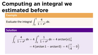
  • 64. Computing an integral we estimated before Example ∫ 1 4 Evaluate the integral dx. 0 1 + x2
  • 65. Example ∫ 1 4 Es mate dx using M4 . 0 1 + x2 Solu on ( ) 1 4 4 4 4 M4 = + + + 4 1 + (1/8)2 1 + (3/8)2 1 + (5/8)2 1 + (7/8)2 ( ) 1 4 4 4 4 = + + + 4 65/64 73/64 89/64 113/64 64 64 64 64 = + + + ≈ 3.1468 65 73 89 113
  • 66. Computing an integral we estimated before Example ∫ 1 4 Evaluate the integral dx. 0 1 + x2 Solu on ∫ 1 ∫ 1 4 1 dx = 4 dx 0 1 + x2 0 1 + x2
  • 67. Computing an integral we estimated before Example ∫ 1 4 Evaluate the integral dx. 0 1 + x2 Solu on ∫ 1 ∫ 1 4 1 dx = 4 dx = 4 arctan(x)|1 0 0 1 + x2 0 1 + x2
  • 68. Computing an integral we estimated before Example ∫ 1 4 Evaluate the integral dx. 0 1 + x2 Solu on ∫ 1 ∫ 1 4 1 dx = 4 dx = 4 arctan(x)|1 0 0 1 + x2 0 1 + x2 = 4 (arctan 1 − arctan 0)
  • 69. Computing an integral we estimated before Example ∫ 1 4 Evaluate the integral dx. 0 1 + x2 Solu on ∫ 1 ∫ 1 4 1 dx = 4 dx = 4 arctan(x)|1 0 1 + x2 0 1+x 2 0 (π ) = 4 (arctan 1 − arctan 0) = 4 −0 4
  • 70. Computing an integral we estimated before Example ∫ 1 4 Evaluate the integral dx. 0 1 + x2 Solu on ∫ 1 ∫ 1 4 1 dx = 4 dx = 4 arctan(x)|1 0 1 + x2 0 1+x 2 0 (π ) = 4 (arctan 1 − arctan 0) = 4 −0 =π 4
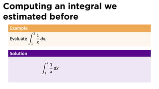
  • 71. Computing an integral we estimated before Example ∫ 2 1 Evaluate dx. 1 x
  • 72. Example ∫ 2 1 Es mate dx using the comparison proper es. 1 x Solu on Since 1 1 1 ≤ ≤ 2 x 1 for all x in [1, 2], we have ∫ 2 1 1 ·1≤ dx ≤ 1 · 1 2 1 x
  • 73. Computing an integral we estimated before Example ∫ 2 1 Evaluate dx. 1 x Solu on ∫ 2 1 dx 1 x
  • 74. Computing an integral we estimated before Example ∫ 2 1 Evaluate dx. 1 x Solu on ∫ 2 1 dx = ln x|2 1 1 x
  • 75. Computing an integral we estimated before Example ∫ 2 1 Evaluate dx. 1 x Solu on ∫ 2 1 dx = ln x|2 = ln 2 − ln 1 1 1 x
  • 76. Computing an integral we estimated before Example ∫ 2 1 Evaluate dx. 1 x Solu on ∫ 2 1 dx = ln x|2 = ln 2 − ln 1 = ln 2 1 1 x
  • 77. Outline Last me: The Definite Integral The definite integral as a limit Proper es of the integral Evalua ng Definite Integrals Examples The Integral as Net Change Indefinite Integrals My first table of integrals Compu ng Area with integrals
  • 78. The Integral as Net Change Another way to state this theorem is: ∫ b F′ (x) dx = F(b) − F(a), a or the integral of a deriva ve along an interval is the net change over that interval. This has many interpreta ons.
  • 79. The Integral as Net Change
  • 80. The Integral as Net Change Corollary If v(t) represents the velocity of a par cle moving rec linearly, then ∫ t1 v(t) dt = s(t1 ) − s(t0 ). t0
  • 81. The Integral as Net Change Corollary If MC(x) represents the marginal cost of making x units of a product, then ∫ x C(x) = C(0) + MC(q) dq. 0
  • 82. The Integral as Net Change Corollary If ρ(x) represents the density of a thin rod at a distance of x from its end, then the mass of the rod up to x is ∫ x m(x) = ρ(s) ds. 0
  • 83. Outline Last me: The Definite Integral The definite integral as a limit Proper es of the integral Evalua ng Definite Integrals Examples The Integral as Net Change Indefinite Integrals My first table of integrals Compu ng Area with integrals
  • 84. A new notation for antiderivatives To emphasize the rela onship between an differen a on and integra on, we use the indefinite integral nota on ∫ f(x) dx for any func on whose deriva ve is f(x).
  • 85. A new notation for antiderivatives To emphasize the rela onship between an differen a on and integra on, we use the indefinite integral nota on ∫ f(x) dx for any func on whose deriva ve is f(x). Thus ∫ x2 dx = 1 x3 + C. 3
  • 86. My first table of integrals . ∫ ∫ ∫ [f(x) + g(x)] dx = f(x) dx + g(x) dx ∫ ∫ ∫ xn+1 xn dx = + C (n ̸= −1) cf(x) dx = c f(x) dx ∫ n+1 ∫ 1 ex dx = ex + C dx = ln |x| + C ∫ ∫ x ax sin x dx = − cos x + C ax dx = +C ∫ ln a ∫ cos x dx = sin x + C csc2 x dx = − cot x + C ∫ ∫ sec2 x dx = tan x + C csc x cot x dx = − csc x + C ∫ ∫ 1 sec x tan x dx = sec x + C √ dx = arcsin x + C ∫ 1 − x2 1 dx = arctan x + C 1 + x2
  • 87. Outline Last me: The Definite Integral The definite integral as a limit Proper es of the integral Evalua ng Definite Integrals Examples The Integral as Net Change Indefinite Integrals My first table of integrals Compu ng Area with integrals
  • 88. Computing Area with integrals Example Find the area of the region bounded by the lines x = 1, x = 4, the x-axis, and the curve y = ex .
  • 89. Computing Area with integrals Example Find the area of the region bounded by the lines x = 1, x = 4, the x-axis, and the curve y = ex . Solu on The answer is ∫ 4 ex dx = ex |4 = e4 − e. 1 1
  • 90. Computing Area with integrals Example Find the area of the region bounded by the curve y = arcsin x, the x-axis, and the line x = 1.
  • 91. Computing Area with integrals Example Find the area of the region bounded by the curve y = arcsin x, the x-axis, and the line x = 1. Solu on y ∫ 1 The answer is arcsin x dx, but π/2 0 we do not know an an deriva ve for arcsin. . x 1
  • 92. Computing Area with integrals Example Find the area of the region bounded by the curve y = arcsin x, the x-axis, and the line x = 1. Solu on y Instead compute the area as π/2 ∫ π/2 π − sin y dy 2 0 . x 1
  • 93. Computing Area with integrals Example Find the area of the region bounded by the curve y = arcsin x, the x-axis, and the line x = 1. Solu on y Instead compute the area as π/2 ∫ π/2 π π π/2 − sin y dy = −[− cos x]0 2 0 2 . x 1
  • 94. Computing Area with integrals Example Find the area of the region bounded by the curve y = arcsin x, the x-axis, and the line x = 1. Solu on y Instead compute the area as π/2 ∫ π/2 π π π/2 π − sin y dy = −[− cos x]0 = −1 2 0 2 2 . x 1
  • 95. Example Find the area between the graph of y = (x − 1)(x − 2), the x-axis, and the ver cal lines x = 0 and x = 3.
  • 96. Example Find the area between the graph of y = (x − 1)(x − 2), the x-axis, and the ver cal lines x = 0 and x = 3. Solu on No ce the func on y = (x − 1)(x − 2) is posi ve on [0, 1) y and (2, 3], and nega ve on (1, 2). . x 1 2 3
  • 97. Example Find the area between the graph of y = (x − 1)(x − 2), the x-axis, and the ver cal lines x = 0 and x = 3. Solu on ∫ 1 A= (x2 − 3x + 2) dx y 0 ∫ 2 − (x2 − 3x + 2) dx 1 ∫ 3 . x + (x2 − 3x + 2) dx 1 2 3 2
  • 98. Example Find the area between the graph of y = (x − 1)(x − 2), the x-axis, and the ver cal lines x = 0 and x = 3. Solu on ∫ 1 A= (x − 1)(x − 2) dx y 0 ∫ 2 − (x − 1)(x − 2) dx 1 ∫ 3 . x + (x − 1)(x − 2) dx 1 2 3 2
  • 99. Example Find the area between the graph of y = (x − 1)(x − 2), the x-axis, and the ver cal lines x = 0 and x = 3. Solu on [1 ]1 y A= 3 x − 3 x2 + 2x 0 3 2 [1 3 3 2 ]2 − 3x − 2x + 2x 1 [ ]3 + 1 x3 − 3 x2 + 3 2 2x 2 . x 11 1 2 3 = 6
  • 100. Interpretation of “negative area” in motion There is an analog in rectlinear mo on: ∫ t1 v(t) dt is net distance traveled. t0 ∫ t1 |v(t)| dt is total distance traveled. t0
  • 101. What about the constant? It seems we forgot about the +C when we say for instance ∫ 1 1 x4 1 1 3 x dx = = −0= 0 4 0 4 4 But no ce [ 4 ]1 ( ) x 1 1 1 +C = + C − (0 + C) = + C − C = 4 0 4 4 4 no ma er what C is. So in an differen a on for definite integrals, the constant is immaterial.
  • 102. Summary The second Fundamental Theorem of Calculus: ∫ b f(x) dx = F(b) − F(a) a where F′ = f. Definite integrals represent net change of a func on over an interval. ∫ We write an deriva ves as indefinite integrals f(x) dx