SlideShare a Scribd company logo
Introduction to Statistical
                                                                                   Machine Learning

                                                                                       c 2011
                                                                                 Christfried Webers
                                                                                       NICTA
                                                                               The Australian National
                                                                                     University

Introduction to Statistical Machine Learning

                         Christfried Webers

                      Statistical Machine Learning Group
                                     NICTA
                                      and
                College of Engineering and Computer Science
                      The Australian National University


                            Canberra
                       February – June 2011


 (Many figures from C. M. Bishop, "Pattern Recognition and Machine Learning")


                                                                                                  1of 197
Introduction to Statistical
                          Machine Learning

                              c 2011
                        Christfried Webers
                              NICTA
                      The Australian National
                            University


      Part V
                      Linear Basis Function
                      Models

                      Maximum Likelihood and

Linear Regression 1   Least Squares

                      Geometry of Least
                      Squares

                      Sequential Learning

                      Regularized Least
                      Squares

                      Multiple Outputs

                      Loss Function for
                      Regression

                      The Bias-Variance
                      Decomposition


                                       159of 197
Introduction to Statistical

Regression                                                             Machine Learning

                                                                           c 2011
                                                                     Christfried Webers
                                                                           NICTA
                                                                   The Australian National
                                                                         University


    Given a training data set of N observations {xn } and target
    values tn .
    Goal : Learn to predict the value of one ore more target
    values t given a new value of the input x.                     Linear Basis Function
                                                                   Models
    Example: Polynomial curve fitting (see Introduction).           Maximum Likelihood and
                                                                   Least Squares

                t                                                  Geometry of Least
                                                                   Squares

                                                                   Sequential Learning

                                                                   Regularized Least
                                                                   Squares

                                                                   Multiple Outputs
                              ?                                    Loss Function for
                                                                   Regression

                                                                   The Bias-Variance
                                                                   Decomposition
                                              x


                                                                                    160of 197
Introduction to Statistical

Supervised Learning                                             Machine Learning

                                                                    c 2011
                                                              Christfried Webers
                                                                    NICTA
                                                            The Australian National
     Training Phase                                               University


          training       model with adjustable
           data x           parameter w

                                                            Linear Basis Function
                                                            Models
          training                                          Maximum Likelihood and
          targets                                           Least Squares
              t
                                                            Geometry of Least
                                                            Squares

                                                            Sequential Learning
                      fix the most appropriate w*            Regularized Least
                                                            Squares
     Test Phase
                                                            Multiple Outputs

                                                            Loss Function for
                                                            Regression
                                                    test
            test            model with fixed
                                                   target   The Bias-Variance
           data x            parameter w*                   Decomposition
                                                      t


                                                                             161of 197
Introduction to Statistical

Linear Basis Function Models                                    Machine Learning

                                                                    c 2011
                                                              Christfried Webers
                                                                    NICTA
                                                            The Australian National
                                                                  University


    Linear combination of fixed nonlinear basis functions
                                M−1                         Linear Basis Function
                                                            Models
                    y(x, w) =         wj φj (x) = wT φ(x)   Maximum Likelihood and
                                                            Least Squares
                                j=0
                                                            Geometry of Least
                                                            Squares
                                         T
    parameter w = (w0 , . . . , wM−1 )                      Sequential Learning

    basis functions φ = (φ0 , . . . , φM−1 )T               Regularized Least
                                                            Squares

    convention φ0 (x) = 1                                   Multiple Outputs

    w0 is the bias parameter                                Loss Function for
                                                            Regression

                                                            The Bias-Variance
                                                            Decomposition


                                                                             162of 197
Introduction to Statistical

Polynomial Basis Functions                                           Machine Learning

                                                                         c 2011
                                                                   Christfried Webers
                                                                         NICTA
    Scalar input variable x                                      The Australian National
                                                                       University

                              φj (x) = xj
    Limitation : Polynomials are global functions of the input
    variable x.
    Extension: Split the input space into regions and fit a       Linear Basis Function
    different polynomial to each region (spline functions).      Models

                                                                 Maximum Likelihood and
                                                                 Least Squares
                    1                                            Geometry of Least
                                                                 Squares

                                                                 Sequential Learning
                   0.5
                                                                 Regularized Least
                                                                 Squares

                                                                 Multiple Outputs
                    0
                                                                 Loss Function for
                                                                 Regression

                 −0.5                                            The Bias-Variance
                                                                 Decomposition


                   −1
                    −1             0          1

                                                                                  163of 197
Introduction to Statistical

’Gaussian’ Basis Functions                                      Machine Learning

                                                                    c 2011
                                                              Christfried Webers
                                                                    NICTA
    Scalar input variable x                                 The Australian National
                                                                  University

                                         (x − µj )2
                        φj (x) = exp −
                                            2s2
    Not a probability distribution.
    No normalisation required, taken care of by the model   Linear Basis Function
    parameters w.                                           Models

                                                            Maximum Likelihood and
                                                            Least Squares
                   1                                        Geometry of Least
                                                            Squares

                                                            Sequential Learning
                  0.75
                                                            Regularized Least
                                                            Squares

                                                            Multiple Outputs
                  0.5
                                                            Loss Function for
                                                            Regression

                  0.25                                      The Bias-Variance
                                                            Decomposition


                   0
                       −1          0                  1

                                                                             164of 197
Introduction to Statistical

Sigmoidal Basis Functions                                       Machine Learning

                                                                    c 2011
                                                              Christfried Webers
                                                                    NICTA
    Scalar input variable x                                 The Australian National
                                                                  University
                                      x − µj
                         φj (x) = σ
                                         s
    where σ(a) is the logistic sigmoid function defined by
                                       1                    Linear Basis Function
                         σ(a) =                             Models
                                  1 + exp(−a)               Maximum Likelihood and
                                                            Least Squares
    σ(a) is related to the hyperbolic tangent tanh(a) by    Geometry of Least
    tanh(a) = 2σ(a) − 1.                                    Squares

                                                            Sequential Learning

                    1                                       Regularized Least
                                                            Squares

                                                            Multiple Outputs

                  0.75                                      Loss Function for
                                                            Regression

                                                            The Bias-Variance
                   0.5                                      Decomposition


                  0.25

                    0                                                        165of 197
Introduction to Statistical

Other Basis Functions                                              Machine Learning

                                                                       c 2011
                                                                 Christfried Webers
                                                                       NICTA
                                                               The Australian National
                                                                     University


    Fourier Basis : each basis function represents a specific   Linear Basis Function
                                                               Models
    frequency and has infinite spatial extent.                  Maximum Likelihood and
                                                               Least Squares
    Wavelets : localised in both space and frequency (also
                                                               Geometry of Least
    mutually orthogonal to simplify appliciation).             Squares

                                                               Sequential Learning
    Splines (polynomials restricted to regions of the input
                                                               Regularized Least
    space).                                                    Squares

                                                               Multiple Outputs

                                                               Loss Function for
                                                               Regression

                                                               The Bias-Variance
                                                               Decomposition


                                                                                166of 197
Introduction to Statistical

Maximum Likelihood and Least Squares                                Machine Learning

                                                                        c 2011
                                                                  Christfried Webers
                                                                        NICTA
                                                                The Australian National
                                                                      University


   No special assumption about the basis functions φj (x). In
   the simplest case, one can think of φj (x) = x.
                                                                Linear Basis Function
   Assume target t is given by                                  Models

                                                                Maximum Likelihood and
                       t = y(x, w) +                            Least Squares

                                                                Geometry of Least
                            deterministic   noise               Squares

                                                                Sequential Learning

   where is a zero-mean Gaussian random variable with           Regularized Least
                                                                Squares
   precision (inverse variance) β.                              Multiple Outputs

   Thus                                                         Loss Function for
                                                                Regression
                p(t | x, w, β) = N (t | y(x, w), β −1 )         The Bias-Variance
                                                                Decomposition


                                                                                 167of 197
Introduction to Statistical

Maximum Likelihood and Least Squares                                     Machine Learning

                                                                             c 2011
                                                                       Christfried Webers
                                                                             NICTA
                                                                     The Australian National
   Likelihood of one target t given the data x                             University


                 p(t | x, w, β) = N (t | y(x, w), β −1 )

   Set of inputs X with corresponding target values t.
                                                                     Linear Basis Function
   Assume data are independent and identically distributed           Models

   (i.i.d.) (means : data are drawn independent and from the         Maximum Likelihood and
                                                                     Least Squares
   same distribution). The likelihood of the target t is then        Geometry of Least
                                                                     Squares
                                N                                    Sequential Learning
             p(t | X, w, β) =         N (tn | y(xn , w), β −1 )      Regularized Least
                                                                     Squares
                                n=1
                                                                     Multiple Outputs
                                N
                                                T           −1       Loss Function for
                            =         N (tn | w φ(xn ), β        )   Regression

                                n=1                                  The Bias-Variance
                                                                     Decomposition

   From now on drop the conditioning variable X from the
   notation, as with supervised learning we do not seek to
   model the distribution of the input data.
                                                                                      168of 197
Introduction to Statistical

Maximum Likelihood and Least Squares                                    Machine Learning

                                                                            c 2011
                                                                      Christfried Webers
                                                                            NICTA
                                                                    The Australian National

   Consider the logarithm of the likelihood p(t | w, β) (the              University


   logarithm is a monoton function! )
                        N
     ln p(t | w, β) =         ln N (tn | wT φ(xn ), β −1 )
                                                                    Linear Basis Function
                        n=1                                         Models
                        N
                                       β       β                    Maximum Likelihood and

                  =           ln          exp − (tn − wT φ(xn ))2   Least Squares

                                       2π      2                    Geometry of Least
                        n=1                                         Squares

                        N       N                                   Sequential Learning
                  =       ln β − ln(2π) − βED (w)
                        2       2                                   Regularized Least
                                                                    Squares

                                                                    Multiple Outputs
   where the sum-of-squares error function is
                                                                    Loss Function for
                                                                    Regression
                                       N
                                   1                                The Bias-Variance
                   ED (w) =                  {tn − wT φ(xn )}2 .    Decomposition
                                   2
                                       n=1

   arg maxw ln p(t | w, β) → arg minw ED (w)
                                                                                     169of 197
Introduction to Statistical

Maximum Likelihood and Least Squares                                      Machine Learning

                                                                              c 2011
                                                                        Christfried Webers
                                                                              NICTA
                                                                      The Australian National
                                                                            University


   Rewrite the Error Function
                    N
               1                               1
      ED (w) =           {tn − wT φ(xn )}2 =     (t − Φw)T (t − Φw)   Linear Basis Function
               2                               2                      Models
                   n=1
                                                                      Maximum Likelihood and
                                                                      Least Squares
                            T
   where t = (t1 , . . . , tN ) , and                                 Geometry of Least
                                                                      Squares
                                                           
                       φ0 (x1 ) φ1 (x1 )   ...    φM−1 (x1 )          Sequential Learning

                     φ0 (x2 ) φ1 (x2 )    ...    φM−1 (x2 )         Regularized Least
                                                                      Squares
                                                            
            Φ= .                     .    ..        .
                     .               .              .               Multiple Outputs
                     .               .       .      .       
                                                                     Loss Function for
                                                                    Regression

                       φ0 (xN ) φ1 (xN )   ...    φM−1 (xN )          The Bias-Variance
                                                                      Decomposition


                                                                                       170of 197
Introduction to Statistical

Maximum Likelihood and Least Squares                                 Machine Learning

                                                                         c 2011
                                                                   Christfried Webers
                                                                         NICTA
   The log likelihood is now                                     The Australian National
                                                                       University

                  N            N
    ln p(t | w, β) =ln β −       ln(2π) − βED (w)
                  2            2
                  N            N           1
                 = ln β −        ln(2π) − β (t − Φw)T (t − Φw)
                  2            2           2                     Linear Basis Function
                                                                 Models
   Find critical points of ln p(t | w, β).                       Maximum Likelihood and
                                                                 Least Squares
   Directional derivative in direction ξ
                                                                 Geometry of Least
                                                                 Squares
              D ln p(t | w, β)(ξ) = βξ T (ΦT t − ΦT Φw)          Sequential Learning

                                                                 Regularized Least
   shall be zero in all directions ξ. Therefore                  Squares

                                                                 Multiple Outputs
                           0 = ΦT t − ΦT Φw,                     Loss Function for
                                                                 Regression

   which results in                                              The Bias-Variance
                                                                 Decomposition


                       wML = (ΦT Φ)−1 ΦT t = Φ† t

   where Φ† is the Moore-Penrose pseudo-inverse of the
   matrix Φ.                                                                      171of 197
Introduction to Statistical

Maximum Likelihood and Least Squares                                     Machine Learning

                                                                             c 2011
                                                                       Christfried Webers
                                                                             NICTA
   Found a critical point wML for ln p(t | w, β). Is it a maximum,   The Australian National
                                                                           University
   a minimum, or a saddle point?
   Calculate the second directional derivative
              D2 ln p(t | w, β)(ξ, ξ) = −β ξ T ΦT Φξ
                                    = −β (Φξ)T Φξ                    Linear Basis Function
                                                                     Models
                                                2
                                    = −β Φξ         ≤0               Maximum Likelihood and
                                                                     Least Squares

                                                                     Geometry of Least
   We found a maximum.                                               Squares

   (Is it enough to check the second directional derivative in       Sequential Learning

   two directions ξ which are the same? Yes, because for any         Regularized Least
                                                                     Squares
   bilinear function g(ξ, η), symmetric in its arguments,            Multiple Outputs

                                                                     Loss Function for
     1                                                               Regression
       [g(ξ, ξ) + g(η, η) − g(ξ − η, ξ − η)]
     2                                                               The Bias-Variance
                                                                     Decomposition
       1
    = [g(ξ, ξ) + g(η, η) − g(ξ, ξ) − g(η, η) + g(ξ, η) + g(η, ξ)]
       2
       1
    = [g(ξ, η) + g(η, ξ)] = g(ξ, η)
       2
                                                                                      172of 197
Introduction to Statistical

Maximum Likelihood and Least Squares                           Machine Learning

                                                                   c 2011
                                                             Christfried Webers
                                                                   NICTA
                                                           The Australian National
   The log likelihood is now                                     University


        ln p(t | wML , β)
            N          N   1
        = ln β − ln(2π) − β (t − ΦwML )T (t − ΦwML )
            2           2  2                               Linear Basis Function
                                                           Models

   Find critical points of ln p(t | w, β)                  Maximum Likelihood and
                                                           Least Squares


                         ∂ ln p(t | wML , β)               Geometry of Least
                                                           Squares
                                             =0
                                 ∂β                        Sequential Learning

                                                           Regularized Least
                                                           Squares
   results in
                                                           Multiple Outputs

                   1   1                                   Loss Function for
                      = (t − ΦwML )T (t − ΦwML )           Regression
                  βML  N                                   The Bias-Variance
                                                           Decomposition

   Note: We can first find the maximum likelihood for w as
   this does not depend on β. Then we can use wML to find
   the maximum likelihood solution for β.
                                                                            173of 197
Introduction to Statistical

Geometry of Least Squares                                                        Machine Learning

                                                                                     c 2011
                                                                               Christfried Webers
                                                                                     NICTA
                                                                             The Australian National
                                                                                   University

    Target vector t = (t1 , . . . , tN )T ∈ RN
    Basis vectors
    ϕj = (Φj1 , . . . , ΦjN )T = (φj (x1 ), . . . , φj (xN ))T ∈ RN span a
    subspace S
                                                                             Linear Basis Function
    Find w such that y = (y(x1 , w), . . . , y(xN , w))T ∈ S is closest      Models

                                                                             Maximum Likelihood and
    to t.                                                                    Least Squares

                                                                             Geometry of Least
                                                                             Squares
                        S
                                                                             Sequential Learning
                                                          t                  Regularized Least
                                                                             Squares
                                             ϕ2                              Multiple Outputs
                         ϕ1        y                                         Loss Function for
                                                                             Regression

                                                                             The Bias-Variance
                                                                             Decomposition


                                                                                              174of 197
Introduction to Statistical

Sequential Learning - Stochastic Gradient                                      Machine Learning

                                                                                   c 2011

Descent                                                                      Christfried Webers
                                                                                   NICTA
                                                                           The Australian National
                                                                                 University


    For large data sets, calculating the maximum likelihood
    parameters wML and βML may be costly.
                                                                           Linear Basis Function
    For real-time applications, never all data in memory.                  Models

                                                                           Maximum Likelihood and
    Use a sequential algorithms (online algorithm).                        Least Squares

                                                                           Geometry of Least
    If the error function is a sum over data points E =         n   En ,   Squares
    then                                                                   Sequential Learning

      1   initialise w(0) to some starting value                           Regularized Least
                                                                           Squares
      2   update the parameter vector at iteration τ + 1 by
                                                                           Multiple Outputs

                               (τ +1)    (τ )                              Loss Function for
                             w          =w      − η En ,                   Regression

                                                                           The Bias-Variance
          where En is the error function after presenting the nth data     Decomposition

          set, and η is the learning rate.


                                                                                            175of 197
Introduction to Statistical

Sequential Learning - Stochastic Gradient                                     Machine Learning

                                                                                  c 2011

Descent                                                                     Christfried Webers
                                                                                  NICTA
                                                                          The Australian National
                                                                                University


    For the sum-of-squares error function, stochastic gradient            Linear Basis Function
                                                                          Models
    descent results in                                                    Maximum Likelihood and
                                                                          Least Squares
                (τ +1)        (τ )                (τ )T
            w            =w          − η tn − w           φ(xn ) φ(xn )   Geometry of Least
                                                                          Squares

                                                                          Sequential Learning
    The value for the learning rate must be chosen carefully. A           Regularized Least
                                                                          Squares
    too large learning rate may prevent the algorithm from
                                                                          Multiple Outputs
    converging. A too small learning rate does follow the data
                                                                          Loss Function for
    too slowly.                                                           Regression

                                                                          The Bias-Variance
                                                                          Decomposition


                                                                                           176of 197
Introduction to Statistical

Regularized Least Squares                                   Machine Learning

                                                                c 2011
                                                          Christfried Webers
                                                                NICTA
                                                        The Australian National
                                                              University


    Add regularisation in order to prevent overfitting

                         ED (w) + λEW (w)
                                                        Linear Basis Function
                                                        Models

    with regularisation coefficient λ.                   Maximum Likelihood and
                                                        Least Squares
    Simple quadratic regulariser                        Geometry of Least
                                                        Squares

                                         1 T            Sequential Learning
                          EW (w) =         w w
                                         2              Regularized Least
                                                        Squares

                                                        Multiple Outputs
    Maximum likelihood solution
                                                        Loss Function for
                                                        Regression
                                     T     −1     T
                      w = λI + Φ Φ               Φ t    The Bias-Variance
                                                        Decomposition


                                                                         177of 197
Introduction to Statistical

Regularized Least Squares                                          Machine Learning

                                                                       c 2011
                                                                 Christfried Webers
                                                                       NICTA
                                                               The Australian National
                                                                     University


    More general regulariser
                                       M
                                   1
                        EW (w) =             |wj |q
                                   2                           Linear Basis Function
                                       j=1                     Models

                                                               Maximum Likelihood and
    q = 1 (lasso) leads to a sparse model if λ large enough.   Least Squares

                                                               Geometry of Least
                                                               Squares

                                                               Sequential Learning

                                                               Regularized Least
                                                               Squares

                                                               Multiple Outputs

                                                               Loss Function for
                                                               Regression

                                                               The Bias-Variance
                                                               Decomposition
    q = 0.5           q=1                    q=2        q=4


                                                                                178of 197
Introduction to Statistical

Comparison of Quadratic and Lasso Regulariser                            Machine Learning

                                                                             c 2011
                                                                       Christfried Webers
                                                                             NICTA
                                                                     The Australian National
                                                                           University

   Assume a sufficiently large regularisation coefficient λ.

  Quadratic regulariser            Lasso regulariser
                     M                            M
             1                                1                      Linear Basis Function
                         w2
                          j                             |wj |        Models
             2                                2                      Maximum Likelihood and
                 j=1                              j=1                Least Squares

        w2                               w2                          Geometry of Least
                                                                     Squares

                                                                     Sequential Learning

                                                                     Regularized Least
                                                                     Squares

                                                                     Multiple Outputs

                                                                     Loss Function for
                                                                     Regression
                 w                            w
                                                                     The Bias-Variance
                                                                     Decomposition


                              w1                                w1


                                                                                      179of 197
Introduction to Statistical

Multiple Outputs                                                       Machine Learning

                                                                           c 2011
                                                                     Christfried Webers
                                                                           NICTA
                                                                   The Australian National
                                                                         University


    More than 1 target variable per data point.
    y becomes a vector instead of a scalar. Each dimension
    can be treated with a different set of basis functions (and
    that may be necessary if the data in the different target      Linear Basis Function
                                                                   Models
    dimensions represent very different types of information.)     Maximum Likelihood and
                                                                   Least Squares
    Here we restrict ourselves to the SAME basis functions         Geometry of Least
                                                                   Squares

                         y(x, w) = WT φ(x)                         Sequential Learning

                                                                   Regularized Least
                                                                   Squares
    where y is a K-dimensional column vector, WT is an M × K       Multiple Outputs
    matrix of model parameters, and                                Loss Function for
    φ(x) = (φ0 (x), . . . , φM−1 (x), φ0 (x) = 1, as before.       Regression

                                                                   The Bias-Variance
    Define target matrix T containing the target vector tT in the
                                                        n
                                                                   Decomposition

    nth row.


                                                                                    180of 197
Introduction to Statistical

Multiple Outputs                                                                Machine Learning

                                                                                    c 2011
                                                                              Christfried Webers
                                                                                    NICTA
                                                                            The Australian National
                                                                                  University


    Suppose the conditional distribution of the target vector is
    an isotropic Gaussian of the form
                                                                            Linear Basis Function
                p(t | x, W, β) = N (t | WT φ(x), β −1 I).                   Models

                                                                            Maximum Likelihood and
                                                                            Least Squares
    The log likelihood is then
                                                                            Geometry of Least
                                                                            Squares
                           N                                                Sequential Learning
     ln p(T | X, W, β) =         ln N (tn | WT φ(xn ), β −1 VI)             Regularized Least
                                                                            Squares
                           n=1
                                                                            Multiple Outputs
                                                   N
                        NK            β       β                   T     2   Loss Function for
                      =    ln               −           tn − W φ(xn )       Regression
                         2            2π      2
                                                  n=1                       The Bias-Variance
                                                                            Decomposition


                                                                                             181of 197
Introduction to Statistical

Multiple Outputs                                                    Machine Learning

                                                                        c 2011
                                                                  Christfried Webers
                                                                        NICTA
                                                                The Australian National
                                                                      University

    Maximisation with respect to W results in

                       WML = (ΦT Φ)−1 ΦT T.

    For each target variable tk , we get                        Linear Basis Function
                                                                Models

                                                                Maximum Likelihood and
                    wk = (ΦT Φ)−1 ΦT tk = Φ† tk .               Least Squares

                                                                Geometry of Least
                                                                Squares
    The solution between the different target variables
                                                                Sequential Learning
    decouples.                                                  Regularized Least
                                                                Squares
    Holds also for a general Gaussian noise distribution with
                                                                Multiple Outputs
    arbitrary covariance matrix.                                Loss Function for
                                                                Regression
    Why? W defines the mean of the Gaussian noise
                                                                The Bias-Variance
    distribution. And the maximum likelihood solution for the   Decomposition

    mean of a multivariate Gaussian is independent of the
    covariance.

                                                                                 182of 197
Introduction to Statistical

Loss Function for Regression                                         Machine Learning

                                                                         c 2011
                                                                   Christfried Webers
                                                                         NICTA
                                                                 The Australian National
                                                                       University


    Over-fitting results from a large number of basis functions   Linear Basis Function
                                                                 Models
    and a relatively small training set.                         Maximum Likelihood and
                                                                 Least Squares
    Regularisation can prevent overfitting, but how to find the    Geometry of Least
    correct value for the regularisation constant λ ?            Squares

                                                                 Sequential Learning
    Frequentists viewpoint of the model complexity is the
                                                                 Regularized Least
    bias-variance trade-off.                                     Squares

                                                                 Multiple Outputs

                                                                 Loss Function for
                                                                 Regression

                                                                 The Bias-Variance
                                                                 Decomposition


                                                                                  183of 197
Introduction to Statistical

Loss Function for Regression                                          Machine Learning

                                                                          c 2011
                                                                    Christfried Webers
                                                                          NICTA
                                                                  The Australian National
                                                                        University
    Choose an estimator y(x) to estimate the target value t for
    each input x.
    Choose a loss function L(t, y(x)) which measures the
    difference between the target t and the estimate y(x).
                                                                  Linear Basis Function
    The expected loss is then                                     Models

                                                                  Maximum Likelihood and
                                                                  Least Squares
                 E [L] =        L(t, y(x)) p(x, t) dx dt          Geometry of Least
                                                                  Squares

                                                                  Sequential Learning
    Common choice: Squared Loss                                   Regularized Least
                                                                  Squares
                                               2
                      L(t, y(x)) = {y(x) − t} .                   Multiple Outputs

                                                                  Loss Function for
                                                                  Regression
    Expected loss for squared loss function                       The Bias-Variance
                                                                  Decomposition

                                          2
               E [L] =       {y(x) − t} p(x, t) dx dt.


                                                                                   184of 197
Introduction to Statistical

Loss Function for Regression                                           Machine Learning

                                                                           c 2011
                                                                     Christfried Webers
                                                                           NICTA
                                                                   The Australian National
                                                                         University


    Expected loss for squared loss function
                                                                   Linear Basis Function
                                         2                         Models
                E [L] =       {y(x) − t} p(x, t) dx dt.
                                                                   Maximum Likelihood and
                                                                   Least Squares

    Minimise E [L] by choosing the regression function             Geometry of Least
                                                                   Squares

                                                                   Sequential Learning
                     t p(x, t) dt                                  Regularized Least
           y(x) =                 =   t p(t | x) dt = Et [t | x]   Squares
                       p(x)
                                                                   Multiple Outputs

                                                                   Loss Function for
    (use calculus of variations to derive this result).            Regression

                                                                   The Bias-Variance
                                                                   Decomposition


                                                                                    185of 197
Introduction to Statistical

Loss Function for Regression                                    Machine Learning

                                                                    c 2011
                                                              Christfried Webers
                                                                    NICTA
                                                            The Australian National
                                                                  University


    The regression function which minimises the expected
    squared loss, is given by the mean of the conditional
    distribution p(t | x).
                                                            Linear Basis Function
                                                            Models

                 t                                          Maximum Likelihood and
                                                            Least Squares

                                               y(x)         Geometry of Least
                                                            Squares

                                                            Sequential Learning
            y(x0 )                                          Regularized Least
                                    p(t|x0 )                Squares

                                                            Multiple Outputs

                                                            Loss Function for
                                                            Regression

                                                            The Bias-Variance
                               x0                     x     Decomposition


                                                                             186of 197
Introduction to Statistical

Loss Function for Regression                                               Machine Learning

                                                                               c 2011
                                                                         Christfried Webers
                                                                               NICTA
                                                                       The Australian National
                                                                             University


    Analyse the expected loss

                                             2
                 E [L] =          {y(x) − t} p(x, t) dx dt.
                                                                       Linear Basis Function
                                                                       Models
    Rewrite the squared loss                                           Maximum Likelihood and
                                                                       Least Squares
                      2                                       2
            {y(x) − t} = {y(x) − E [t | x] + E [t | x] − t}            Geometry of Least
                                                                       Squares
                                                 2                 2
                          = {y(x) − E [t | x]} + {E [t | x] − t}       Sequential Learning

                                                                       Regularized Least
                          + 2 {y(x) − E [t | x]} {E [t | x] − t}       Squares

                                                                       Multiple Outputs

    Claim                                                              Loss Function for
                                                                       Regression

                                                                       The Bias-Variance
               {y(x) − E [t | x]} {E [t | x] − t} p(x, t) dx dt = 0.   Decomposition


                                                                                        187of 197
Introduction to Statistical

Loss Function for Regression                                                   Machine Learning

                                                                                   c 2011
                                                                             Christfried Webers
                                                                                   NICTA
                                                                           The Australian National
                                                                                 University
    Claim

              {y(x) − E [t | x]} {E [t | x] − t} p(x, t) dx dt = 0.

    Seperate functions depending on t from function                        Linear Basis Function
                                                                           Models
    depending on x                                                         Maximum Likelihood and
                                                                           Least Squares

                                                                           Geometry of Least
            {y(x) − E [t | x]}      {E [t | x] − t} p(x, t) dt   dx        Squares

                                                                           Sequential Learning

                                                                           Regularized Least
    Calculate the integral over t                                          Squares

                                                                           Multiple Outputs

                                                            t p(x, t)      Loss Function for
       {E [t | x] − t} p(x, t) dt = E [t | x] p(x) − p(x)             dt   Regression

                                                               p(x)        The Bias-Variance
                                                                           Decomposition
                                 = E [t | x] p(x) − p(x)E [t | x]
                                 =0

                                                                                            188of 197
Introduction to Statistical

Loss Function for Regression                                            Machine Learning

                                                                            c 2011
                                                                      Christfried Webers
                                                                            NICTA
                                                                    The Australian National
                                                                          University


    The expected loss is now
                                                                    Linear Basis Function
                                                                    Models
                                2
      E [L] =   {y(x) − E [t | x]} p(x) dx +   var[t | x] p(x) dx   Maximum Likelihood and
                                                                    Least Squares

                                                                    Geometry of Least
                                                                    Squares
    Minimise first term by choosing appropriate y(x).
                                                                    Sequential Learning
    Second term represents the intrinsic variability of the         Regularized Least
                                                                    Squares
    target data (can be regarded as noise). Independent of the
                                                                    Multiple Outputs
    choice y(x), can not be reduced by learning a better y(x).
                                                                    Loss Function for
                                                                    Regression

                                                                    The Bias-Variance
                                                                    Decomposition


                                                                                     189of 197
Introduction to Statistical

The Bias-Variance Decomposition                                   Machine Learning

                                                                      c 2011
                                                                Christfried Webers
                                                                      NICTA
                                                              The Australian National
                                                                    University


    Consider now the dependency on the data set D.
    Prediction function now y(x; D).
    Consider again squared loss for which the optimal         Linear Basis Function
                                                              Models
    prediction is given by the conditional expectation h(x)   Maximum Likelihood and
                                                              Least Squares

                                                              Geometry of Least
                   h(x) = E [t | x] =   t p(t | x) dt.        Squares

                                                              Sequential Learning

                                                              Regularized Least
    BUT: we can not know h(x) exactly, as we would need an    Squares

    infinite number of training data to learn it accurately.   Multiple Outputs

                                                              Loss Function for
    Evaluate performance of algorithm by taking the           Regression

    expectation ED [L] over all data sets D                   The Bias-Variance
                                                              Decomposition


                                                                               190of 197
Introduction to Statistical

The Bias-Variance Decomposition                                Machine Learning

                                                                   c 2011
                                                             Christfried Webers
                                                                   NICTA
                                                           The Australian National
                                                                 University


    Taking the expectation over all data sets D

           ED [E [L]] =   ED {y(x; D) − h(x)}2 p(x) dx
                                                           Linear Basis Function
                                                           Models

                     +      {h(x) − t}2 p(x, t) dx dt      Maximum Likelihood and
                                                           Least Squares

                                                           Geometry of Least
                                                           Squares
    Again, add and subtract the expectation ED [y(x; D)]   Sequential Learning

                                                           Regularized Least
           {y(x; D) − h(x)}2 = { y(x; D) − ED [y(x; D)]    Squares

                                                           Multiple Outputs
                                 + ED [y(x; D)] − h(x)}2   Loss Function for
                                                           Regression

    and show that the mixed term does vanish under the     The Bias-Variance
                                                           Decomposition
    expectation ED [. . .].


                                                                            191of 197
Introduction to Statistical

The Bias-Variance Decomposition                                        Machine Learning

                                                                           c 2011
                                                                     Christfried Webers
                                                                           NICTA
                                                                   The Australian National
                                                                         University
    Expected loss ED [L] over all data sets D

            expected loss = (bias)2 + variance + noise.

    where                                                          Linear Basis Function
                                                                   Models

                                            2
         (bias)2 =    {ED [y(x; D)] − h(x)} p(x) dx                Maximum Likelihood and
                                                                   Least Squares

                                                                   Geometry of Least
                                                                   Squares
                                                     2
       variance =     ED {y(x; D) − ED [y(x; D)]}        p(x) dx   Sequential Learning

                                                                   Regularized Least
                                                                   Squares
            noise =     {h(x) − t}2 p(x, t) dx dt.                 Multiple Outputs

                                                                   Loss Function for
                                                                   Regression
    squared bias : how much does the average prediction over
                                                                   The Bias-Variance
    all data sets differ from the desired regression function ?    Decomposition


    variance : how much do solutions for individual data sets
    vary around their average ?

                                                                                    192of 197
Introduction to Statistical

The Bias-Variance Decomposition                                         Machine Learning

                                                                            c 2011
                                                                      Christfried Webers
                                                                            NICTA
                                                                    The Australian National
                                                                          University


Dependence of bias and variance on the model complexity


                                                                    Linear Basis Function
                                                                    Models
       1                                      1
                     ln λ = 2.6                                     Maximum Likelihood and
   t                                      t
                                                                    Least Squares

       0                                      0                     Geometry of Least
                                                                    Squares

                                                                    Sequential Learning
   −1                                     −1                        Regularized Least
                                                                    Squares

           0                          1           0            1    Multiple Outputs
                                  x                        x
                                                                    Loss Function for
Left: Result of fitting the model to 100 data sets, only 25 shown.   Regression

Right: Average of the 100 fits in red, the sinusoidal function       The Bias-Variance
                                                                    Decomposition
from where the data were created in green.


                                                                                     193of 197
Introduction to Statistical

The Bias-Variance Decomposition                                         Machine Learning

                                                                            c 2011
                                                                      Christfried Webers
                                                                            NICTA
                                                                    The Australian National
                                                                          University


Dependence of bias and variance on the model complexity


                                                                    Linear Basis Function
                                                                    Models
       1                                    1
                     ln λ = −0.31
   t                                    t                           Maximum Likelihood and
                                                                    Least Squares

       0                                    0                       Geometry of Least
                                                                    Squares

                                                                    Sequential Learning
   −1                                   −1                          Regularized Least
                                                                    Squares

           0                        1           0              1    Multiple Outputs
                               x                           x
                                                                    Loss Function for
Left: Result of fitting the model to 100 data sets, only 25 shown.   Regression

Right: Average of the 100 fits in red, the sinusoidal function       The Bias-Variance
                                                                    Decomposition
from where the data were created in green.


                                                                                     194of 197
Introduction to Statistical

The Bias-Variance Decomposition                                         Machine Learning

                                                                            c 2011
                                                                      Christfried Webers
                                                                            NICTA
                                                                    The Australian National
                                                                          University


Dependence of bias and variance on the model complexity


                                                                    Linear Basis Function
                                                                    Models
       1                                   1
                     ln λ = −2.4
   t                                   t                            Maximum Likelihood and
                                                                    Least Squares

       0                                   0                        Geometry of Least
                                                                    Squares

                                                                    Sequential Learning
   −1                                  −1                           Regularized Least
                                                                    Squares

           0                       1           0               1    Multiple Outputs
                               x                           x
                                                                    Loss Function for
Left: Result of fitting the model to 100 data sets, only 25 shown.   Regression

Right: Average of the 100 fits in red, the sinusoidal function       The Bias-Variance
                                                                    Decomposition
from where the data were created in green.


                                                                                     195of 197
Introduction to Statistical

The Bias-Variance Decomposition                                  Machine Learning

                                                                     c 2011
                                                               Christfried Webers
                                                                     NICTA
                                                             The Australian National
    Squared bias, variance, their sum, and test data               University


    The minimum for (bias)2 + variance occurs close to the
    value that gives the minimum error

         0.15                                                Linear Basis Function
                                                             Models
                         (bias)2
                                                             Maximum Likelihood and
         0.12            variance                            Least Squares

                         (bias)2 + variance                  Geometry of Least
                                                             Squares
         0.09            test error
                                                             Sequential Learning

                                                             Regularized Least
         0.06                                                Squares

                                                             Multiple Outputs

         0.03                                                Loss Function for
                                                             Regression

                                                             The Bias-Variance
            0                                                Decomposition
            −3      −2         −1             0   1    2
                                    ln λ


                                                                              196of 197
Introduction to Statistical

The Bias-Variance Decomposition                                 Machine Learning

                                                                    c 2011
                                                              Christfried Webers
                                                                    NICTA
                                                            The Australian National
                                                                  University


    Tradeoff between bias and variance                      Linear Basis Function
                                                            Models
        simple models have high bias and low variance
                                                            Maximum Likelihood and
        complex models have low bias and high variance      Least Squares

    The sum of bias and variance has a minimum at some      Geometry of Least
                                                            Squares
    model complexity.                                       Sequential Learning

    The bias-variance decomposition needs many data sets,   Regularized Least
                                                            Squares
    which are not always available.                         Multiple Outputs

                                                            Loss Function for
                                                            Regression

                                                            The Bias-Variance
                                                            Decomposition


                                                                             197of 197

More Related Content

PDF
Classification Based Machine Learning Algorithms
Md. Main Uddin Rony
 
PPTX
Polynomial regression
naveedaliabad
 
ODP
Simple Linear Regression (simplified)
Haoran Zhang
 
PDF
08 linear classification_2
nep_test_account
 
KEY
Random Variables
Tomoki Tsuchida
 
PDF
Linear Regression Algorithm | Linear Regression in Python | Machine Learning ...
Edureka!
 
PPTX
Machine Learning - Simple Linear Regression
Siddharth Shrivastava
 
PPTX
Machine learning session4(linear regression)
Abhimanyu Dwivedi
 
Classification Based Machine Learning Algorithms
Md. Main Uddin Rony
 
Polynomial regression
naveedaliabad
 
Simple Linear Regression (simplified)
Haoran Zhang
 
08 linear classification_2
nep_test_account
 
Random Variables
Tomoki Tsuchida
 
Linear Regression Algorithm | Linear Regression in Python | Machine Learning ...
Edureka!
 
Machine Learning - Simple Linear Regression
Siddharth Shrivastava
 
Machine learning session4(linear regression)
Abhimanyu Dwivedi
 

What's hot (20)

PDF
Autoencoders
CloudxLab
 
PDF
Lecture5 - C4.5
Albert Orriols-Puig
 
PPTX
ML - Simple Linear Regression
Andrew Ferlitsch
 
PDF
Probability Distributions
Anthony J. Evans
 
PDF
2.03 bayesian estimation
Andres Mendez-Vazquez
 
PPTX
Power series & Radius of convergence
Dhruv Darji
 
PPTX
support vector regression
Akhilesh Joshi
 
PPTX
Statistical classification: A review on some techniques
Giorgos Bamparopoulos
 
PPT
Linear regression
vermaumeshverma
 
PDF
Discrete probability distributions
Habibullah Bahar University College
 
PDF
Introduction to Statistical Machine Learning
mahutte
 
PPTX
Negative Binomial Distribution
Suchithra Edakunni
 
PDF
What is the Expectation Maximization (EM) Algorithm?
Kazuki Yoshida
 
PDF
Ridge regression
Ananda Swarup
 
PPTX
Q-Q Plot | Statistics
Transweb Global Inc
 
PPT
Simple lin regress_inference
Kemal İnciroğlu
 
PDF
Assumptions of Linear Regression - Machine Learning
Kush Kulshrestha
 
PDF
Introduction to probability distributions-Statistics and probability analysis
Vijay Hemmadi
 
PDF
Logistic regression
Venkata Reddy Konasani
 
PDF
Statistical inference: Probability and Distribution
Eugene Yan Ziyou
 
Autoencoders
CloudxLab
 
Lecture5 - C4.5
Albert Orriols-Puig
 
ML - Simple Linear Regression
Andrew Ferlitsch
 
Probability Distributions
Anthony J. Evans
 
2.03 bayesian estimation
Andres Mendez-Vazquez
 
Power series & Radius of convergence
Dhruv Darji
 
support vector regression
Akhilesh Joshi
 
Statistical classification: A review on some techniques
Giorgos Bamparopoulos
 
Linear regression
vermaumeshverma
 
Discrete probability distributions
Habibullah Bahar University College
 
Introduction to Statistical Machine Learning
mahutte
 
Negative Binomial Distribution
Suchithra Edakunni
 
What is the Expectation Maximization (EM) Algorithm?
Kazuki Yoshida
 
Ridge regression
Ananda Swarup
 
Q-Q Plot | Statistics
Transweb Global Inc
 
Simple lin regress_inference
Kemal İnciroğlu
 
Assumptions of Linear Regression - Machine Learning
Kush Kulshrestha
 
Introduction to probability distributions-Statistics and probability analysis
Vijay Hemmadi
 
Logistic regression
Venkata Reddy Konasani
 
Statistical inference: Probability and Distribution
Eugene Yan Ziyou
 
Ad

Viewers also liked (6)

PDF
Overview of solutions for machine monitoring
Ivan Zgela
 
PPTX
Theory of machines
Sourabh Kumar
 
PPT
Complex System Engineering
Emmanuel Fuchs
 
PDF
March12 natarajan
BBKuhn
 
PPTX
Faulty radiographs
melbia shine
 
PPSX
FINITE STATE MACHINE AND CHOMSKY HIERARCHY
nishimanglani
 
Overview of solutions for machine monitoring
Ivan Zgela
 
Theory of machines
Sourabh Kumar
 
Complex System Engineering
Emmanuel Fuchs
 
March12 natarajan
BBKuhn
 
Faulty radiographs
melbia shine
 
FINITE STATE MACHINE AND CHOMSKY HIERARCHY
nishimanglani
 
Ad

More from nep_test_account (18)

PDF
Database slide
nep_test_account
 
PDF
database slide 1
nep_test_account
 
PDF
Doc2pages
nep_test_account
 
PDF
Doc2pages
nep_test_account
 
PDF
PDF TEST
nep_test_account
 
PDF
Baboom!
nep_test_account
 
PDF
Baboom!
nep_test_account
 
PDF
test pdf
nep_test_account
 
PDF
linear classification
nep_test_account
 
PDF
Lecture Notes in Machine Learning
nep_test_account
 
PDF
Induction of Decision Trees
nep_test_account
 
PDF
Large-Scale Machine Learning at Twitter
nep_test_account
 
PDF
A Few Useful Things to Know about Machine Learning
nep_test_account
 
PDF
linear regression part 2
nep_test_account
 
PDF
Probability
nep_test_account
 
PDF
Linear Algebra
nep_test_account
 
PDF
Introduction
nep_test_account
 
Database slide
nep_test_account
 
database slide 1
nep_test_account
 
Doc2pages
nep_test_account
 
Doc2pages
nep_test_account
 
linear classification
nep_test_account
 
Lecture Notes in Machine Learning
nep_test_account
 
Induction of Decision Trees
nep_test_account
 
Large-Scale Machine Learning at Twitter
nep_test_account
 
A Few Useful Things to Know about Machine Learning
nep_test_account
 
linear regression part 2
nep_test_account
 
Probability
nep_test_account
 
Linear Algebra
nep_test_account
 
Introduction
nep_test_account
 

Linear Regression

  • 1. Introduction to Statistical Machine Learning c 2011 Christfried Webers NICTA The Australian National University Introduction to Statistical Machine Learning Christfried Webers Statistical Machine Learning Group NICTA and College of Engineering and Computer Science The Australian National University Canberra February – June 2011 (Many figures from C. M. Bishop, "Pattern Recognition and Machine Learning") 1of 197
  • 2. Introduction to Statistical Machine Learning c 2011 Christfried Webers NICTA The Australian National University Part V Linear Basis Function Models Maximum Likelihood and Linear Regression 1 Least Squares Geometry of Least Squares Sequential Learning Regularized Least Squares Multiple Outputs Loss Function for Regression The Bias-Variance Decomposition 159of 197
  • 3. Introduction to Statistical Regression Machine Learning c 2011 Christfried Webers NICTA The Australian National University Given a training data set of N observations {xn } and target values tn . Goal : Learn to predict the value of one ore more target values t given a new value of the input x. Linear Basis Function Models Example: Polynomial curve fitting (see Introduction). Maximum Likelihood and Least Squares t Geometry of Least Squares Sequential Learning Regularized Least Squares Multiple Outputs ? Loss Function for Regression The Bias-Variance Decomposition x 160of 197
  • 4. Introduction to Statistical Supervised Learning Machine Learning c 2011 Christfried Webers NICTA The Australian National Training Phase University training model with adjustable data x parameter w Linear Basis Function Models training Maximum Likelihood and targets Least Squares t Geometry of Least Squares Sequential Learning fix the most appropriate w* Regularized Least Squares Test Phase Multiple Outputs Loss Function for Regression test test model with fixed target The Bias-Variance data x parameter w* Decomposition t 161of 197
  • 5. Introduction to Statistical Linear Basis Function Models Machine Learning c 2011 Christfried Webers NICTA The Australian National University Linear combination of fixed nonlinear basis functions M−1 Linear Basis Function Models y(x, w) = wj φj (x) = wT φ(x) Maximum Likelihood and Least Squares j=0 Geometry of Least Squares T parameter w = (w0 , . . . , wM−1 ) Sequential Learning basis functions φ = (φ0 , . . . , φM−1 )T Regularized Least Squares convention φ0 (x) = 1 Multiple Outputs w0 is the bias parameter Loss Function for Regression The Bias-Variance Decomposition 162of 197
  • 6. Introduction to Statistical Polynomial Basis Functions Machine Learning c 2011 Christfried Webers NICTA Scalar input variable x The Australian National University φj (x) = xj Limitation : Polynomials are global functions of the input variable x. Extension: Split the input space into regions and fit a Linear Basis Function different polynomial to each region (spline functions). Models Maximum Likelihood and Least Squares 1 Geometry of Least Squares Sequential Learning 0.5 Regularized Least Squares Multiple Outputs 0 Loss Function for Regression −0.5 The Bias-Variance Decomposition −1 −1 0 1 163of 197
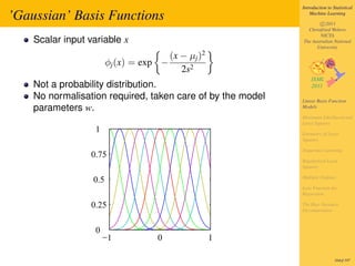
  • 7. Introduction to Statistical ’Gaussian’ Basis Functions Machine Learning c 2011 Christfried Webers NICTA Scalar input variable x The Australian National University (x − µj )2 φj (x) = exp − 2s2 Not a probability distribution. No normalisation required, taken care of by the model Linear Basis Function parameters w. Models Maximum Likelihood and Least Squares 1 Geometry of Least Squares Sequential Learning 0.75 Regularized Least Squares Multiple Outputs 0.5 Loss Function for Regression 0.25 The Bias-Variance Decomposition 0 −1 0 1 164of 197
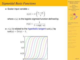
  • 8. Introduction to Statistical Sigmoidal Basis Functions Machine Learning c 2011 Christfried Webers NICTA Scalar input variable x The Australian National University x − µj φj (x) = σ s where σ(a) is the logistic sigmoid function defined by 1 Linear Basis Function σ(a) = Models 1 + exp(−a) Maximum Likelihood and Least Squares σ(a) is related to the hyperbolic tangent tanh(a) by Geometry of Least tanh(a) = 2σ(a) − 1. Squares Sequential Learning 1 Regularized Least Squares Multiple Outputs 0.75 Loss Function for Regression The Bias-Variance 0.5 Decomposition 0.25 0 165of 197
  • 9. Introduction to Statistical Other Basis Functions Machine Learning c 2011 Christfried Webers NICTA The Australian National University Fourier Basis : each basis function represents a specific Linear Basis Function Models frequency and has infinite spatial extent. Maximum Likelihood and Least Squares Wavelets : localised in both space and frequency (also Geometry of Least mutually orthogonal to simplify appliciation). Squares Sequential Learning Splines (polynomials restricted to regions of the input Regularized Least space). Squares Multiple Outputs Loss Function for Regression The Bias-Variance Decomposition 166of 197
  • 10. Introduction to Statistical Maximum Likelihood and Least Squares Machine Learning c 2011 Christfried Webers NICTA The Australian National University No special assumption about the basis functions φj (x). In the simplest case, one can think of φj (x) = x. Linear Basis Function Assume target t is given by Models Maximum Likelihood and t = y(x, w) + Least Squares Geometry of Least deterministic noise Squares Sequential Learning where is a zero-mean Gaussian random variable with Regularized Least Squares precision (inverse variance) β. Multiple Outputs Thus Loss Function for Regression p(t | x, w, β) = N (t | y(x, w), β −1 ) The Bias-Variance Decomposition 167of 197
  • 11. Introduction to Statistical Maximum Likelihood and Least Squares Machine Learning c 2011 Christfried Webers NICTA The Australian National Likelihood of one target t given the data x University p(t | x, w, β) = N (t | y(x, w), β −1 ) Set of inputs X with corresponding target values t. Linear Basis Function Assume data are independent and identically distributed Models (i.i.d.) (means : data are drawn independent and from the Maximum Likelihood and Least Squares same distribution). The likelihood of the target t is then Geometry of Least Squares N Sequential Learning p(t | X, w, β) = N (tn | y(xn , w), β −1 ) Regularized Least Squares n=1 Multiple Outputs N T −1 Loss Function for = N (tn | w φ(xn ), β ) Regression n=1 The Bias-Variance Decomposition From now on drop the conditioning variable X from the notation, as with supervised learning we do not seek to model the distribution of the input data. 168of 197
  • 12. Introduction to Statistical Maximum Likelihood and Least Squares Machine Learning c 2011 Christfried Webers NICTA The Australian National Consider the logarithm of the likelihood p(t | w, β) (the University logarithm is a monoton function! ) N ln p(t | w, β) = ln N (tn | wT φ(xn ), β −1 ) Linear Basis Function n=1 Models N β β Maximum Likelihood and = ln exp − (tn − wT φ(xn ))2 Least Squares 2π 2 Geometry of Least n=1 Squares N N Sequential Learning = ln β − ln(2π) − βED (w) 2 2 Regularized Least Squares Multiple Outputs where the sum-of-squares error function is Loss Function for Regression N 1 The Bias-Variance ED (w) = {tn − wT φ(xn )}2 . Decomposition 2 n=1 arg maxw ln p(t | w, β) → arg minw ED (w) 169of 197
  • 13. Introduction to Statistical Maximum Likelihood and Least Squares Machine Learning c 2011 Christfried Webers NICTA The Australian National University Rewrite the Error Function N 1 1 ED (w) = {tn − wT φ(xn )}2 = (t − Φw)T (t − Φw) Linear Basis Function 2 2 Models n=1 Maximum Likelihood and Least Squares T where t = (t1 , . . . , tN ) , and Geometry of Least Squares   φ0 (x1 ) φ1 (x1 ) ... φM−1 (x1 ) Sequential Learning  φ0 (x2 ) φ1 (x2 ) ... φM−1 (x2 )  Regularized Least Squares   Φ= . . .. .  . . .  Multiple Outputs  . . . .   Loss Function for   Regression φ0 (xN ) φ1 (xN ) ... φM−1 (xN ) The Bias-Variance Decomposition 170of 197
  • 14. Introduction to Statistical Maximum Likelihood and Least Squares Machine Learning c 2011 Christfried Webers NICTA The log likelihood is now The Australian National University N N ln p(t | w, β) =ln β − ln(2π) − βED (w) 2 2 N N 1 = ln β − ln(2π) − β (t − Φw)T (t − Φw) 2 2 2 Linear Basis Function Models Find critical points of ln p(t | w, β). Maximum Likelihood and Least Squares Directional derivative in direction ξ Geometry of Least Squares D ln p(t | w, β)(ξ) = βξ T (ΦT t − ΦT Φw) Sequential Learning Regularized Least shall be zero in all directions ξ. Therefore Squares Multiple Outputs 0 = ΦT t − ΦT Φw, Loss Function for Regression which results in The Bias-Variance Decomposition wML = (ΦT Φ)−1 ΦT t = Φ† t where Φ† is the Moore-Penrose pseudo-inverse of the matrix Φ. 171of 197
  • 15. Introduction to Statistical Maximum Likelihood and Least Squares Machine Learning c 2011 Christfried Webers NICTA Found a critical point wML for ln p(t | w, β). Is it a maximum, The Australian National University a minimum, or a saddle point? Calculate the second directional derivative D2 ln p(t | w, β)(ξ, ξ) = −β ξ T ΦT Φξ = −β (Φξ)T Φξ Linear Basis Function Models 2 = −β Φξ ≤0 Maximum Likelihood and Least Squares Geometry of Least We found a maximum. Squares (Is it enough to check the second directional derivative in Sequential Learning two directions ξ which are the same? Yes, because for any Regularized Least Squares bilinear function g(ξ, η), symmetric in its arguments, Multiple Outputs Loss Function for 1 Regression [g(ξ, ξ) + g(η, η) − g(ξ − η, ξ − η)] 2 The Bias-Variance Decomposition 1 = [g(ξ, ξ) + g(η, η) − g(ξ, ξ) − g(η, η) + g(ξ, η) + g(η, ξ)] 2 1 = [g(ξ, η) + g(η, ξ)] = g(ξ, η) 2 172of 197
  • 16. Introduction to Statistical Maximum Likelihood and Least Squares Machine Learning c 2011 Christfried Webers NICTA The Australian National The log likelihood is now University ln p(t | wML , β) N N 1 = ln β − ln(2π) − β (t − ΦwML )T (t − ΦwML ) 2 2 2 Linear Basis Function Models Find critical points of ln p(t | w, β) Maximum Likelihood and Least Squares ∂ ln p(t | wML , β) Geometry of Least Squares =0 ∂β Sequential Learning Regularized Least Squares results in Multiple Outputs 1 1 Loss Function for = (t − ΦwML )T (t − ΦwML ) Regression βML N The Bias-Variance Decomposition Note: We can first find the maximum likelihood for w as this does not depend on β. Then we can use wML to find the maximum likelihood solution for β. 173of 197
  • 17. Introduction to Statistical Geometry of Least Squares Machine Learning c 2011 Christfried Webers NICTA The Australian National University Target vector t = (t1 , . . . , tN )T ∈ RN Basis vectors ϕj = (Φj1 , . . . , ΦjN )T = (φj (x1 ), . . . , φj (xN ))T ∈ RN span a subspace S Linear Basis Function Find w such that y = (y(x1 , w), . . . , y(xN , w))T ∈ S is closest Models Maximum Likelihood and to t. Least Squares Geometry of Least Squares S Sequential Learning t Regularized Least Squares ϕ2 Multiple Outputs ϕ1 y Loss Function for Regression The Bias-Variance Decomposition 174of 197
  • 18. Introduction to Statistical Sequential Learning - Stochastic Gradient Machine Learning c 2011 Descent Christfried Webers NICTA The Australian National University For large data sets, calculating the maximum likelihood parameters wML and βML may be costly. Linear Basis Function For real-time applications, never all data in memory. Models Maximum Likelihood and Use a sequential algorithms (online algorithm). Least Squares Geometry of Least If the error function is a sum over data points E = n En , Squares then Sequential Learning 1 initialise w(0) to some starting value Regularized Least Squares 2 update the parameter vector at iteration τ + 1 by Multiple Outputs (τ +1) (τ ) Loss Function for w =w − η En , Regression The Bias-Variance where En is the error function after presenting the nth data Decomposition set, and η is the learning rate. 175of 197
  • 19. Introduction to Statistical Sequential Learning - Stochastic Gradient Machine Learning c 2011 Descent Christfried Webers NICTA The Australian National University For the sum-of-squares error function, stochastic gradient Linear Basis Function Models descent results in Maximum Likelihood and Least Squares (τ +1) (τ ) (τ )T w =w − η tn − w φ(xn ) φ(xn ) Geometry of Least Squares Sequential Learning The value for the learning rate must be chosen carefully. A Regularized Least Squares too large learning rate may prevent the algorithm from Multiple Outputs converging. A too small learning rate does follow the data Loss Function for too slowly. Regression The Bias-Variance Decomposition 176of 197
  • 20. Introduction to Statistical Regularized Least Squares Machine Learning c 2011 Christfried Webers NICTA The Australian National University Add regularisation in order to prevent overfitting ED (w) + λEW (w) Linear Basis Function Models with regularisation coefficient λ. Maximum Likelihood and Least Squares Simple quadratic regulariser Geometry of Least Squares 1 T Sequential Learning EW (w) = w w 2 Regularized Least Squares Multiple Outputs Maximum likelihood solution Loss Function for Regression T −1 T w = λI + Φ Φ Φ t The Bias-Variance Decomposition 177of 197
  • 21. Introduction to Statistical Regularized Least Squares Machine Learning c 2011 Christfried Webers NICTA The Australian National University More general regulariser M 1 EW (w) = |wj |q 2 Linear Basis Function j=1 Models Maximum Likelihood and q = 1 (lasso) leads to a sparse model if λ large enough. Least Squares Geometry of Least Squares Sequential Learning Regularized Least Squares Multiple Outputs Loss Function for Regression The Bias-Variance Decomposition q = 0.5 q=1 q=2 q=4 178of 197
  • 22. Introduction to Statistical Comparison of Quadratic and Lasso Regulariser Machine Learning c 2011 Christfried Webers NICTA The Australian National University Assume a sufficiently large regularisation coefficient λ. Quadratic regulariser Lasso regulariser M M 1 1 Linear Basis Function w2 j |wj | Models 2 2 Maximum Likelihood and j=1 j=1 Least Squares w2 w2 Geometry of Least Squares Sequential Learning Regularized Least Squares Multiple Outputs Loss Function for Regression w w The Bias-Variance Decomposition w1 w1 179of 197
  • 23. Introduction to Statistical Multiple Outputs Machine Learning c 2011 Christfried Webers NICTA The Australian National University More than 1 target variable per data point. y becomes a vector instead of a scalar. Each dimension can be treated with a different set of basis functions (and that may be necessary if the data in the different target Linear Basis Function Models dimensions represent very different types of information.) Maximum Likelihood and Least Squares Here we restrict ourselves to the SAME basis functions Geometry of Least Squares y(x, w) = WT φ(x) Sequential Learning Regularized Least Squares where y is a K-dimensional column vector, WT is an M × K Multiple Outputs matrix of model parameters, and Loss Function for φ(x) = (φ0 (x), . . . , φM−1 (x), φ0 (x) = 1, as before. Regression The Bias-Variance Define target matrix T containing the target vector tT in the n Decomposition nth row. 180of 197
  • 24. Introduction to Statistical Multiple Outputs Machine Learning c 2011 Christfried Webers NICTA The Australian National University Suppose the conditional distribution of the target vector is an isotropic Gaussian of the form Linear Basis Function p(t | x, W, β) = N (t | WT φ(x), β −1 I). Models Maximum Likelihood and Least Squares The log likelihood is then Geometry of Least Squares N Sequential Learning ln p(T | X, W, β) = ln N (tn | WT φ(xn ), β −1 VI) Regularized Least Squares n=1 Multiple Outputs N NK β β T 2 Loss Function for = ln − tn − W φ(xn ) Regression 2 2π 2 n=1 The Bias-Variance Decomposition 181of 197
  • 25. Introduction to Statistical Multiple Outputs Machine Learning c 2011 Christfried Webers NICTA The Australian National University Maximisation with respect to W results in WML = (ΦT Φ)−1 ΦT T. For each target variable tk , we get Linear Basis Function Models Maximum Likelihood and wk = (ΦT Φ)−1 ΦT tk = Φ† tk . Least Squares Geometry of Least Squares The solution between the different target variables Sequential Learning decouples. Regularized Least Squares Holds also for a general Gaussian noise distribution with Multiple Outputs arbitrary covariance matrix. Loss Function for Regression Why? W defines the mean of the Gaussian noise The Bias-Variance distribution. And the maximum likelihood solution for the Decomposition mean of a multivariate Gaussian is independent of the covariance. 182of 197
  • 26. Introduction to Statistical Loss Function for Regression Machine Learning c 2011 Christfried Webers NICTA The Australian National University Over-fitting results from a large number of basis functions Linear Basis Function Models and a relatively small training set. Maximum Likelihood and Least Squares Regularisation can prevent overfitting, but how to find the Geometry of Least correct value for the regularisation constant λ ? Squares Sequential Learning Frequentists viewpoint of the model complexity is the Regularized Least bias-variance trade-off. Squares Multiple Outputs Loss Function for Regression The Bias-Variance Decomposition 183of 197
  • 27. Introduction to Statistical Loss Function for Regression Machine Learning c 2011 Christfried Webers NICTA The Australian National University Choose an estimator y(x) to estimate the target value t for each input x. Choose a loss function L(t, y(x)) which measures the difference between the target t and the estimate y(x). Linear Basis Function The expected loss is then Models Maximum Likelihood and Least Squares E [L] = L(t, y(x)) p(x, t) dx dt Geometry of Least Squares Sequential Learning Common choice: Squared Loss Regularized Least Squares 2 L(t, y(x)) = {y(x) − t} . Multiple Outputs Loss Function for Regression Expected loss for squared loss function The Bias-Variance Decomposition 2 E [L] = {y(x) − t} p(x, t) dx dt. 184of 197
  • 28. Introduction to Statistical Loss Function for Regression Machine Learning c 2011 Christfried Webers NICTA The Australian National University Expected loss for squared loss function Linear Basis Function 2 Models E [L] = {y(x) − t} p(x, t) dx dt. Maximum Likelihood and Least Squares Minimise E [L] by choosing the regression function Geometry of Least Squares Sequential Learning t p(x, t) dt Regularized Least y(x) = = t p(t | x) dt = Et [t | x] Squares p(x) Multiple Outputs Loss Function for (use calculus of variations to derive this result). Regression The Bias-Variance Decomposition 185of 197
  • 29. Introduction to Statistical Loss Function for Regression Machine Learning c 2011 Christfried Webers NICTA The Australian National University The regression function which minimises the expected squared loss, is given by the mean of the conditional distribution p(t | x). Linear Basis Function Models t Maximum Likelihood and Least Squares y(x) Geometry of Least Squares Sequential Learning y(x0 ) Regularized Least p(t|x0 ) Squares Multiple Outputs Loss Function for Regression The Bias-Variance x0 x Decomposition 186of 197
  • 30. Introduction to Statistical Loss Function for Regression Machine Learning c 2011 Christfried Webers NICTA The Australian National University Analyse the expected loss 2 E [L] = {y(x) − t} p(x, t) dx dt. Linear Basis Function Models Rewrite the squared loss Maximum Likelihood and Least Squares 2 2 {y(x) − t} = {y(x) − E [t | x] + E [t | x] − t} Geometry of Least Squares 2 2 = {y(x) − E [t | x]} + {E [t | x] − t} Sequential Learning Regularized Least + 2 {y(x) − E [t | x]} {E [t | x] − t} Squares Multiple Outputs Claim Loss Function for Regression The Bias-Variance {y(x) − E [t | x]} {E [t | x] − t} p(x, t) dx dt = 0. Decomposition 187of 197
  • 31. Introduction to Statistical Loss Function for Regression Machine Learning c 2011 Christfried Webers NICTA The Australian National University Claim {y(x) − E [t | x]} {E [t | x] − t} p(x, t) dx dt = 0. Seperate functions depending on t from function Linear Basis Function Models depending on x Maximum Likelihood and Least Squares Geometry of Least {y(x) − E [t | x]} {E [t | x] − t} p(x, t) dt dx Squares Sequential Learning Regularized Least Calculate the integral over t Squares Multiple Outputs t p(x, t) Loss Function for {E [t | x] − t} p(x, t) dt = E [t | x] p(x) − p(x) dt Regression p(x) The Bias-Variance Decomposition = E [t | x] p(x) − p(x)E [t | x] =0 188of 197
  • 32. Introduction to Statistical Loss Function for Regression Machine Learning c 2011 Christfried Webers NICTA The Australian National University The expected loss is now Linear Basis Function Models 2 E [L] = {y(x) − E [t | x]} p(x) dx + var[t | x] p(x) dx Maximum Likelihood and Least Squares Geometry of Least Squares Minimise first term by choosing appropriate y(x). Sequential Learning Second term represents the intrinsic variability of the Regularized Least Squares target data (can be regarded as noise). Independent of the Multiple Outputs choice y(x), can not be reduced by learning a better y(x). Loss Function for Regression The Bias-Variance Decomposition 189of 197
  • 33. Introduction to Statistical The Bias-Variance Decomposition Machine Learning c 2011 Christfried Webers NICTA The Australian National University Consider now the dependency on the data set D. Prediction function now y(x; D). Consider again squared loss for which the optimal Linear Basis Function Models prediction is given by the conditional expectation h(x) Maximum Likelihood and Least Squares Geometry of Least h(x) = E [t | x] = t p(t | x) dt. Squares Sequential Learning Regularized Least BUT: we can not know h(x) exactly, as we would need an Squares infinite number of training data to learn it accurately. Multiple Outputs Loss Function for Evaluate performance of algorithm by taking the Regression expectation ED [L] over all data sets D The Bias-Variance Decomposition 190of 197
  • 34. Introduction to Statistical The Bias-Variance Decomposition Machine Learning c 2011 Christfried Webers NICTA The Australian National University Taking the expectation over all data sets D ED [E [L]] = ED {y(x; D) − h(x)}2 p(x) dx Linear Basis Function Models + {h(x) − t}2 p(x, t) dx dt Maximum Likelihood and Least Squares Geometry of Least Squares Again, add and subtract the expectation ED [y(x; D)] Sequential Learning Regularized Least {y(x; D) − h(x)}2 = { y(x; D) − ED [y(x; D)] Squares Multiple Outputs + ED [y(x; D)] − h(x)}2 Loss Function for Regression and show that the mixed term does vanish under the The Bias-Variance Decomposition expectation ED [. . .]. 191of 197
  • 35. Introduction to Statistical The Bias-Variance Decomposition Machine Learning c 2011 Christfried Webers NICTA The Australian National University Expected loss ED [L] over all data sets D expected loss = (bias)2 + variance + noise. where Linear Basis Function Models 2 (bias)2 = {ED [y(x; D)] − h(x)} p(x) dx Maximum Likelihood and Least Squares Geometry of Least Squares 2 variance = ED {y(x; D) − ED [y(x; D)]} p(x) dx Sequential Learning Regularized Least Squares noise = {h(x) − t}2 p(x, t) dx dt. Multiple Outputs Loss Function for Regression squared bias : how much does the average prediction over The Bias-Variance all data sets differ from the desired regression function ? Decomposition variance : how much do solutions for individual data sets vary around their average ? 192of 197
  • 36. Introduction to Statistical The Bias-Variance Decomposition Machine Learning c 2011 Christfried Webers NICTA The Australian National University Dependence of bias and variance on the model complexity Linear Basis Function Models 1 1 ln λ = 2.6 Maximum Likelihood and t t Least Squares 0 0 Geometry of Least Squares Sequential Learning −1 −1 Regularized Least Squares 0 1 0 1 Multiple Outputs x x Loss Function for Left: Result of fitting the model to 100 data sets, only 25 shown. Regression Right: Average of the 100 fits in red, the sinusoidal function The Bias-Variance Decomposition from where the data were created in green. 193of 197
  • 37. Introduction to Statistical The Bias-Variance Decomposition Machine Learning c 2011 Christfried Webers NICTA The Australian National University Dependence of bias and variance on the model complexity Linear Basis Function Models 1 1 ln λ = −0.31 t t Maximum Likelihood and Least Squares 0 0 Geometry of Least Squares Sequential Learning −1 −1 Regularized Least Squares 0 1 0 1 Multiple Outputs x x Loss Function for Left: Result of fitting the model to 100 data sets, only 25 shown. Regression Right: Average of the 100 fits in red, the sinusoidal function The Bias-Variance Decomposition from where the data were created in green. 194of 197
  • 38. Introduction to Statistical The Bias-Variance Decomposition Machine Learning c 2011 Christfried Webers NICTA The Australian National University Dependence of bias and variance on the model complexity Linear Basis Function Models 1 1 ln λ = −2.4 t t Maximum Likelihood and Least Squares 0 0 Geometry of Least Squares Sequential Learning −1 −1 Regularized Least Squares 0 1 0 1 Multiple Outputs x x Loss Function for Left: Result of fitting the model to 100 data sets, only 25 shown. Regression Right: Average of the 100 fits in red, the sinusoidal function The Bias-Variance Decomposition from where the data were created in green. 195of 197
  • 39. Introduction to Statistical The Bias-Variance Decomposition Machine Learning c 2011 Christfried Webers NICTA The Australian National Squared bias, variance, their sum, and test data University The minimum for (bias)2 + variance occurs close to the value that gives the minimum error 0.15 Linear Basis Function Models (bias)2 Maximum Likelihood and 0.12 variance Least Squares (bias)2 + variance Geometry of Least Squares 0.09 test error Sequential Learning Regularized Least 0.06 Squares Multiple Outputs 0.03 Loss Function for Regression The Bias-Variance 0 Decomposition −3 −2 −1 0 1 2 ln λ 196of 197
  • 40. Introduction to Statistical The Bias-Variance Decomposition Machine Learning c 2011 Christfried Webers NICTA The Australian National University Tradeoff between bias and variance Linear Basis Function Models simple models have high bias and low variance Maximum Likelihood and complex models have low bias and high variance Least Squares The sum of bias and variance has a minimum at some Geometry of Least Squares model complexity. Sequential Learning The bias-variance decomposition needs many data sets, Regularized Least Squares which are not always available. Multiple Outputs Loss Function for Regression The Bias-Variance Decomposition 197of 197