Linear regression.ppt

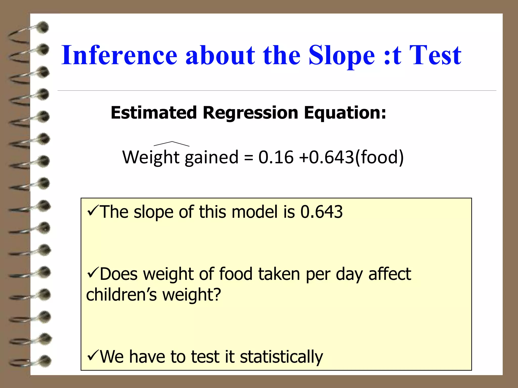
University of Gondar
College of medicine and health science
Department of Epidemiology and
Biostatistics
Linear regression
Lemma Derseh (BSc., MPH)

Scatter Plots and Correlation
 Before trying to fit any model it is better to see its scatter plot
 A scatter plot (or scatter diagram) is used to show the
relationship between two variables
 If a scatter plot once show some sort of linear relationship, we
can use correlation analysis to measure the strength of linear
relationship between two variables
o Only concerned with strength of linear relationship and its
direction
o We consider the two variables equally; as a result no causal
effect is implied

Scatter Plot Examples
y
x
y
x
y
y
x
x
Linear relationships Curvilinear relationships

y
x
y
x
y
y
x
x
Strong relationships
Weak relationships

y
x
y
x
No relationship at all

Correlation Coefficient
 The population correlation coefficient ρ (rho) measures
the strength of the association between the variables
 The sample correlation coefficient r is an estimate of ρ
and is used to measure the strength of the linear
relationship in the sample observations

Features of ρ and r
 Unit free
 Range between -1 and 1
 The closer to -1, the stronger the negative linear
relationship
 The closer to 1, the stronger the positive linear relationship
 The closer to 0, the weaker the linear relationship

r = +0.3 r = +1
Examples of Approximate r Values
y
x
y
x
y
x
y
x
y
x
r = -1 r = -.6 r = 0

Calculating the Correlation Coefficient
yy
xx
xy SS
SS
SS
y
y
x
x
y
y
x
x
r /
]
)
(
][
)
(
[
)
)(
(
2
2









where:
r = Sample correlation coefficient
n = Sample size
x = Value of the ‘independent’ variable
y = Value of the ‘dependent’ variable
   
  




]
)
(
)
(
][
)
(
)
(
[ 2
2
2
2
y
y
n
x
x
n
y
x
xy
n
r
Sample correlation coefficient:
or the algebraic equivalent:

Example
Child
Height
(cm)
Child
Weight
(Kg)
x y xy x2 y2
35 8 280 1225 64
49 9 441 2401 81
27 7 189 729 49
33 6 198 1089 36
60 13 780 3600 169
21 7 147 441 49
45 11 495 2025 121
51 12 612 2601 144
=321 =73 =3142 =14111 =713

0
10
20
30
40
50
60
70
0 2 4 6 8 10 12 14
0.886
]
(321)
][8(14111)
(73)
[8(713)
(73)(321)
8(3142)
]
y)
(
)
y
][n(
x)
(
)
x
[n(
y
x
xy
n
r
2
2
2
2
2
2









   
  
Child weight, x
Child
Height,
y
Calculation Example
r = 0.886 → relatively strong positive
linear association between x and y

SPSS out put
SPSS Correlation Output
Analyze /correlate /bivariate /pearson /OK
Correlation between Child height and weight
Correlations
Child
weight
Child
height
Child Weight Pearson Correlation 1 0.886
Sig. (2-tailed) 0.003
N 8 8
Child height Pearson Correlation 0.886 1
Sig. (2-tailed) 0.003
N 8 8

Significance Test for Correlation
 Hypotheses
H0: ρ = 0 (no correlation)
HA: ρ ≠ 0 (correlation exists)
 Test statistic (with n – 2 degrees of freedom)
2
n
r
1
r
t
2



Here, the degree of freedom is taken to be n-2
because, two points can be joined by a straight line
surely

Example:
Is there evidence of a linear relationship between child
height and weight at the 0.05 level of significance?
H0: ρ = 0 (No correlation)
H1: ρ ≠ 0 (correlation exists)
 = 0.05 , df = 8 - 2 = 6
4.68
2
8
.886
1
.886
2
n
r
1
r
t
2
2








Introduction to Regression Analysis
 Regression analysis is used to:
Predict the value of a dependent variable based on the
value of at least one independent variable
Explain the impact of changes in an independent
variable on the dependent variable
 Dependent variable: the variable we wish to explain. In
linear regression it is always continuous variable
 Independent variable: the variable used to explain the
dependent variable. In linear regression it could have any
measurement scale have any measurement scale.

Simple Linear Regression Model
 Only one independent variable, x
 Relationship between x and y is described
by a linear function
 Changes in y are assumed to be caused by
changes in x

ε
x
β
β
y 1
0 


Linear component
Population Linear Regression
The population regression model:
Population
y intercept
Population
Slope
Coefficient
Random
Error
term, or
residual
Dependent
Variable Independent
Variable
Random Error
component

Linear Regression Assumptions
 The relationship between the two variables, x and y is Linear
 Independent observations
 Error values are Normally distributed for any given value of x
 The probability distribution of the errors has Equal variance
 Fixed independent variables (not random = non-stochastic = given
values = deterministic); the only randomness in the values of Y
comes from the error term 
 No autocorrelation of the errors (has some similarities with the 2nd)
 No outlier distortion

Assumptions viewed pictorially
LINE (Liner, Independent, Normal and Equal
variance) assumptions
my|x= +  x
~N(my|x s2
y|x)
Y
X
Identical normal
distributions of
errors, all centered on
the regression line.

Population Linear Regression
Random Error
for this x value
y
x
Observed
Value of y
for xi
Predicted
Value of y
for xi
ε
x
β
β
y 1
0 


xi
Slope = β1
Intercept
= β0
εi

x
b
b
ŷ 1
0
i 

The sample regression line provides an estimate of the
population regression line
Estimated Regression Model
Estimate of
the regression
intercept
Estimate of the
regression slope
Estimated
(or predicted)
y value
Independent
variable
The individual random error terms ei have a mean of zero

Least Squares Criterion
 b0 and b1 are obtained by finding the values of b0 and
b1 that minimize the sum of the squared residuals
2
1
0
2
2
x))
b
(b
(y
)
ŷ
(y
e









The Least Squares Equation
 After some application of calculus (derivation)
and equating it to zero, we can find the
following:
 
  



n
x
x
n
y
x
xy
b 2
2
1
)
(





 2
1
)
(
)
)(
(
x
x
y
y
x
x
b
x
b
y
b 1
0 

and

 b0 is the estimated average value of y when the
value of x is zero (provided that x is inside the data
range considered).
 Otherwise it shows the portion of the variability of
the dependent variable left unexplained by the
independent variables considered
 b1 is the estimated change in the average value of y
as a result of a one-unit change in x
Interpretation of the Slope and the Intercept

Example: Simple Linear Regression
 A researcher wishes to examine the relationship between
the amount of the daily average diets taken by a cohort of
20 sample children and the weight gained by them in one
month (both measured in kg). The content of the food is the
same for all of them.
 Dependent variable (y) = weight gained in one month
measured in kilogram
 Independent variable (x) = average weight of diet taken per
day by a child measured in Kilogram

Sample Data for child weight Model
Weight gained (y)
Diet (x) Weight gained (y) Diet (x)
0.4 0.65 0.86 1.1
0.46 0.66 0.89 1.12
0.55 0.63 0.91 1.20
0.56 0.73 0.93 1.32
0.65 0.78 0.96 1.33
0.67 0.76 0.98 1.35
0.78 0.72 1.02 1.42
0.79 0.84 1.04 1.1
0.80 0.87 1.08 1.5
0.83 0.97 1.11 1.3

Estimation using the computational formula
 
  



n
x
x
n
y
x
xy
b 2
2
1
)
(
From the data we have:
Σx = 20.35, Σy = 16.27, Σxy = 17.58, Σx2 = 22.30
643
.
0
20
/
12
.
414
30
.
22
20
/
27
.
16
*
35
.
20
57
.
17
1 



b
160
.
0
0175
.
1
*
643
.
0
8135
.
0
1
0 



 x
b
y
b

Regression Using SPSS
Analyze/ regression/linear….
Coefficients
Model
Unstandardized Coefficients
Standardized
Coefficients
t Sig.
B Std. Error Beta
(Constant) 0.160 .077 2.065 .054
foodweight 0.643 .073 .900 8.772 .000
Weight gained = 0.16 +0.643(food weight)

Interpretation of the Intercept, b0
 Here, no child had had 0 kilogram of food per day, so for
foods within the range of sizes observed, 0.16Kg is the
portion of the weight gained not explained by food.
 Whereas, b1 = 0.643 tells us that the average weight of a
child increases by 0.643, on average, for each additional
one kilogram of food taken each day
Weight gained = 0.16 + 0.643(food weight)

Explained and Unexplained Variation
Total variation is made up of two parts:
SSE
SSR
SST 

Total sum of
Squares
Sum of Squares
Regression
Sum of Squares
Error
 
 2
)
y
y
(
SST  
 2
)
ŷ
y
(
SSE
 
 2
)
y
ŷ
(
SSR
where:
= Average value of the dependent variable
y = Observed values of the dependent variable
= Estimated value of y for the given x value
ŷ
y

Xi
y
x
yi
SST = (yi - y)2
SSE = (yi - yi )2

SSR = (yi - y)2

_
_
_
Explained and Unexplained …
y

y
y
_
Y


 The coefficient of determination is the portion of the total
variation in the dependent variable that is explained by
variation in the independent variable
 The coefficient of determination is also called R-squared and
is denoted as R2
Coefficient of Determination, R2
1
R
0 2


where
squares
of
sum
total
regression
by
explained
squares
of
sum
SST
SSR
R 

2

Coefficient of Determination, R2
In the single independent variable case, the coefficient
of determination is
Where:
R2 = Coefficient of determination
r = Simple correlation coefficient
2
2
r
R 

Coefficient of Determination, R2 cont…
 The F-test testes the statistical significance of the
regression of the dependent variable on the
independent variable: H0: β = 0
 However, the reliability of the regression equation is
very commonly measured by the correlation
coefficient R.
 Equivalently one can check the statistical
significance of R or R2 using F-test and can reach
exactly the same F-value as model coefficients’ test

SPSS output
Model R R Square
Adjusted R
Square
1 0.900 0.810 0.800
ANOVA
Model
Sum of
Squares df
Mean
Square F Sig.
Regression 0.658 1 0.658 76.948 .000
Residual 0.154 18 0.009
Total 0.812 19
0.81
0.812
0.658
SST
SSR
R2



Model summary
81% of the variation in
children’s weight
increment is explained
by variation in food
weight they took

SPSS output
R R Square
Adjusted R
Square
Std. Error of the estimate
(the standard deviation of errors)
0.900 0.810 0.800 0.09248
Coefficients
Model
Unstandardized
Coefficients
Standardized
Coefficients
t Sig.
B Std. Error Beta
(Constant) 0.160 0.077 2.065 .054
foodweight 0.643 0.073 0.900 8.772 .000
ANOVA
Model
Sum of
Squares df
Mean
Square F Sig.
Regression 0.658 1 0.658 76.948 0.000
Residual 0.154 18 0.009
Total 0.812 19
Root of ‘mean square error’ = SƐ
Model summary

Inference about the Slope: t-Test
 t test for a population slope
Is there a linear relationship between x and y?
 Null and alternative hypotheses
H0: β1 = 0 (no linear relationship)
H1: β1  0 (linear relationship does exist)
 Test statistic
– 1
b
1
1
s
β
b
t

 2
n
d.f. 

Where:
b1 = Sample regression slope (coefficient)
β1 = Hypothesized slope, usually 0
sb1 = Estimator of the standard error of the slope

Estimated Regression Equation:
The slope of this model is 0.643
Does weight of food taken per day affect
children’s weight?
We have to test it statistically
Inference about the Slope :t Test
Weight gained = 0.16 +0.643(food)

Inferences about the Slope: t-Test
Example
Conclusion: There is
sufficient evidence that food
weight taken per day affects
children’s weight
1
b
s
b1
Coefficients
Model
Unstandardized
Coefficients
Standardized
Coefficients
t Sig.
B Std. Error Beta
(Constant) 0.160 0.077 2.065 .054
Food weight 0.643 0.073 0.900 8.772 0.000
The calculated t-test is 8.772
which is greater than the
tabulated one 2.074
Decision: Reject Ho
1
b
1
s
0
b
t



Confidence Interval estimation
Coefficients
Model
Unstandardized
Coefficients
Standardized
Coefficients
t Sig.
95% Confidence
Interval for B
B
Std.
Error Beta
Lower
Bound
Upper
Bound
(Constant) 0.160 0.077 2.065 .054 -0.003 0.322
Food weight 0.643 0.073 0.900 8.772 0.000 0.489 0.796
Confidence Interval Estimate of the Slope:
df = n-2 = 18, t(0.025,18) = 2.101
1
b
/2
1 s
t
b 

The 95% confidence interval for the slope is (0.489, 0.796).
Note also that this 95% confidence interval does not include 0.
Look the relationship between all the figures in the blue circles

Multiple linear regression
Multiple Linear Regression (MLR) is a
statistical method for estimating the
relationship between a dependent variable
and two or more independent (or predictor)
variables.
Function: Ypred = a + b1X1 + B2X2 +… + BnXn

Multiple Linear Regression
Simply, MLR is a method for studying the
relationship between a dependent variable
and two or more independent variables.
Purposes:
Prediction
Explanation
Theory building

Predictable variation by
the combination of
independent variables
Variations
Total Variation in Y
Unpredictable
Variation

44
Assumptions of the Linear regression Model
1. Linear Functional form
2. Fixed independent variables
3. Independent observations
4. Representative sample and proper specification of the model
(no omitted variables)*
5. Normality of the residuals or errors
6. Equality of variance of the errors (homogeneity of residual
variance)
7. No multicollinearity*
8. No autocorrelation of the errors
9. No outlier distortion
(Most of them, except the 4th and 7th, are mentioned in the simple
linear regression model assumptions)

Multiple Coefficient of Determination, R2
o In multiple regression ,the corresponding correlation
coefficient is called Multiple Correlation Coefficient
 Since there are more than one independent variables, multiple
correlation coefficient R is the correlation between the
observed y and predicted y values while it is between x and y
in the case of r (simple correlation)
 Unlike the situation for simple correlation, 0 < R < 1, because
it would be impossible to have a negative correlation between
the observed and the least-squares predicted values
 The square of a multiple correlation coefficient is of course the
corresponding coefficient of determination


Intercorrelation or collinearlity
 If the two independent variables are uncorrelated, we
can uniquely partition the amount of variance in Y due
to X1 and X2 and bias is avoided.
 Small inter-correlations between the independent
variables will not greatly bias the b coefficients.
 However, large inter-correlations will bias the b
coefficients and for this reason other mathematical
procedures are needed

Multiple regression
%fat age Sex
9.5 23.0 0.0
27.9 23.0 1.0
7.8 27.0 0.0
17.8 27.0 0.0
31.4 39.0 1.0
25.9 41.0 1.0
27.4 45.0 0.0
25.2 49.0 1.0
31.1 50.0 1.0
34.7 53.0 1.0
42.0 53.0 1.0
42.0 54.0 1.0
29.1 54.0 1.0
32.5 56.0 1.0
30.3 57.0 1.0
21.0 57.0 1.0
33.0 58.0 1.0
33.8 58.0 1.0
41.1 60.0 1.0
34.5 61.0 1.0
Example:
Regress the percentage of fat relative
to body on age and sex
SPSS result on the next slide!

Model Summary
Model R
R
Square
Adjusted R
Square
Std. Error of
the Estimate
Change Statistics
R Square
Change F Change df1 df2
Sig. F
Change
1 .729a .532 .506 6.5656 .532 20.440 1 18 .000
2 .794b .631 .587 5.9986 .099 4.564 1 17 .047
a. Predictors: (Constant), sex; b. Predictors: (Constant), sex, age
ANOVA
Model Sum of Squares df Mean Square F Sig.
1 Regression 881.128 1 881.128 20.440 .000a
Residual 775.932 18 43.107
Total 1657.060 19
2 Regression 1045.346 2 522.673 14.525 .000b
Residual 611.714 17 35.983
Total 1657.060 19
a. Predictors: (Constant), sex; b. Predictors: (Constant), sex, age; c. Dependent Variable: %age of body fat
Coefficients
Model
Unstandardized Coefficients
Standardized
Coefficients
t Sig.
95% Confidence
Interval for B
B Std. Error Beta
Lower
Bound
Upper
Bound
1 (Constant) 15.625 3.283 4.760 .000 8.728 22.522
sex 16.594 3.670 .729 4.521 .000 8.883 24.305
2 (Constant) 6.209 5.331 1.165 .260 -5.039 17.457
sex 10.130 4.517 .445 2.243 .039 .600 19.659
age .309 .145 .424 2.136 .047 .004 .614
a. Dependent Variable: %age of body fat relative to body

Linear regression.ppt

More Related Content

What's hot

Similar to Linear regression.ppt

More from habtamu biazin

Recently uploaded

In this document

Linear regression.ppt