Machine learning introduction lecture notes

CS 179: LECTURE 13
INTRO TO MACHINE LEARNING

GOALS OF WEEKS 5-6
 What is machine learning (ML) and when is it useful?
 Intro to major techniques and applications
 Give examples
 How can CUDA help?
 Departure from usual pattern: we will give the
application first, and the CUDA later

HOW TO FOLLOW THIS LECTURE
 This lecture and the next one will have a lot of math!
 Don’t worry about keeping up with the derivations 100%
 Important equations will be boxed
 Key terms to understand: loss/objective function, linear
regression, gradient descent, linear classifier
 The theory lectures will probably be boring for those of
you who have done some machine learning (CS156/155)
already

WHAT IS ML GOOD FOR?
 Handwriting recognition
 Spam detection

WHAT IS ML GOOD FOR?
 Teaching a robot how to do a backflip
 https://youtu.be/fRj34o4hN4I
 Predicting the performance of a stock portfolio
 The list goes on!

WHAT IS ML?
 What do these problems have in common?
 Some pattern we want to learn
 No good closed-form model for it
 LOTS of data
 What can we do?
 Use data to learn a statistical model for
the pattern we are interested in

DATA REPRESENTATION
 One data point is a vector 𝑥 in ℝ𝑑
 A 30 × 30 pixel image is a 900-dimensional
vector (one component per pixel intensity)
 If we are classifying an email as spam or not
spam, set 𝑑 = number of words in dictionary
 Count the number of times 𝑛𝑖 that a word 𝑖
appears in an email and set 𝑥𝑖 = 𝑛𝑖
 The possibilities are endless 

WHAT ARE WE TRYING TO DO?
 Given an input 𝑥 ∈ ℝ𝑑
, produce an output 𝑦
 What is 𝑦?
 Could be a real number, e.g. predicted return
of a given stock portfolio
 Could be 0 or 1, e.g. spam or not spam
 Could be a vector in ℝ𝑚
, e.g. telling a robot
how to move each of its 𝑚 joints
 Just like 𝑥, 𝑦 can be almost anything 

EXAMPLE OF (𝑥, 𝑦) PAIRS
 ,
0
0
0
0
0
1
0
0
0
0
, ,
1
0
0
0
0
0
0
0
0
0
, ,
0
1
0
0
0
0
0
0
0
0
, ,
0
0
0
1
0
0
0
0
0
0
, etc.

NOTATION
𝑥′
=
1
𝑥
∈ ℝ𝑑+1
𝐗 = 𝑥 1
, … , 𝑥 𝑁
∈ ℝ𝑑×𝑁
𝐗′
= 𝑥 1 ′
, … , 𝑥 𝑁 ′
∈ ℝ 𝑑+1 ×𝑁
𝐘 = 𝑦 1
, … , 𝑦 𝑁 𝑇
∈ ℝ𝑁×𝑚
𝕀 𝑝 =
1
0
𝑝 is true
otherwise

STATISTICAL MODELS
 Given (𝐗, 𝐘) (𝑁 pairs of 𝑥 𝑖
, 𝑦 𝑖
data), how
do we accurately predict an output 𝑦 given
an input 𝑥?
 One solution: a model 𝑓(𝑥) parametrized by
a vector (or matrix) 𝑤, denoted as 𝑓 𝑥; 𝑤
 The task is finding a set of optimal
parameters 𝑤

FITTING A MODEL
 So what does optimal mean?
 Under some measure of closeness, we want
𝑓(𝑥; 𝑤) to be as close as possible to the true
solution 𝑦 for any input 𝑥
 This measure of closeness is called a loss
function or objective function and is
denoted 𝐽 𝑤; 𝐗, 𝐘 -- it depends on our data
set (𝐗, 𝐘)!
 To fit a model, we try to find parameters 𝑤∗
that minimize 𝐽(𝑤; 𝐗, 𝐘), i.e. an optimal 𝑤

FITTING A MODEL
 What characterizes a good loss function?
 Represents the magnitude of our model’s
error on the data we are given
 Penalizes large errors more than small ones
 Continuous and differentiable in 𝑤
 Bonus points if it is also convex in 𝑤
 Continuity, differentiability, and convexity are
to make minimization easier

LINEAR REGRESSION
 𝑓 𝑥; 𝑤 = 𝑤0 + 𝑖=1
𝑑
𝑤𝑖𝑥𝑖 = 𝑤𝑇
𝑥′
 Below: 𝑑 = 1. 𝑤𝑇
𝑥′ is graphed.

LINEAR REGRESSION
 What should we use as a loss function?
 Each 𝑦 𝑖
is a real number
 Mean-squared error is a good choice 
 𝐽 𝑤; 𝐗, 𝐘 =
1
𝑁 𝑖=1
𝑁
𝑓 𝑥 𝑖
; 𝑤 − 𝑦 𝑖 2
=
1
𝑁 𝑖=1
𝑁
𝑤𝑇
𝑥 𝑖 ′
− 𝑦 𝑖
2
=
1
𝑁
𝑤𝑇
𝐗′ − 𝐘 𝑇
𝑤𝑇
𝐗′
− 𝐘

GRADIENT DESCENT
 How do we find 𝑤∗
= argmin
𝑤∈ℝ𝑑+1
𝐽(𝑤; 𝐗, 𝐘)?
 A function’s gradient points in the direction
of steepest ascent, and its negative in the
direction of steepest descent
 Following the gradient downhill will cause us
to converge to a local minimum!

GRADIENT DESCENT
 Fix some constant learning rate 𝜂 (0.03 is usually a
good place to start)
 Initialize 𝑤 randomly
 Typically select each component of 𝑤 independently
from some standard distribution (uniform, normal, etc.)
 While 𝑤 is still changing (hasn’t converged)
 Update 𝑤 ← 𝑤 − 𝜂∇𝐽 𝑤; 𝐗, 𝐘

GRADIENT DESCENT
 For mean squared error loss in linear regression,
∇𝐽 𝑤; 𝐗, 𝐘 =
2
𝑁
𝑤𝑇
𝐗′
𝐗′𝑇
− 𝐗′
𝐘
 This is just linear algebra! GPUs are good at this kind of
thing 
 Why do we care?
 𝑓 𝑥; 𝑤∗ = 𝑤∗𝑇
𝑥′ is the model with the lowest possible
mean-squared error on our training dataset (𝐗, 𝐘)!

STOCHASTIC GRADIENT DESCENT
 The previous algorithm computes the gradient over the
entire data set before stepping.
 Called batch gradient descent
 What if we just picked a single data point 𝑥 𝑖
, 𝑦 𝑖
at
random, computed the gradient for that point, and
updated the parameters?
 Called stochastic gradient descent

STOCHASTIC GRADIENT DESCENT
 Advantages of SGD
 Easier to implement for large datasets
 Works better for non-convex loss functions
 Sometimes faster
 Often use SGD on a “mini-batch” of 𝑘 examples rather
than just one at a time
 Allows higher throughput and more parallelization

BINARY LINEAR CLASSIFICATION
 𝑓 𝑥; 𝑤 = 𝕀 𝑤𝑇
𝑥′
> 0
 Divides ℝ𝑑
into two half-spaces
 𝑤𝑇
𝑥′
= 0 is a hyperplane
 A line in 2D, a plane in 3D, and so on
 Known as the decision boundary
 Everything on one side of the hyperplane is
class 0 and everything on the other side is
class 1

BINARY LINEAR CLASSIFICATION
 Below: 𝑑 = 2. Black line is the decision boundary
𝑤𝑇
𝑥′ = 0

MULTI-CLASS GENERALIZATION
 We want to classify 𝑥 into one of 𝑚 classes
 For each input 𝑥, 𝑦 is a vector in ℝ𝑚
with 𝑦𝑘 = 1 if class 𝑥 =
𝑘 and 𝑦𝑗 = 0 otherwise (i.e. 𝑦𝑘 = 𝕀 class 𝑥 = 𝑘 )
 Known as a one-hot vector
 Our model 𝑓(𝑥; 𝐖) is parametrized by a 𝑚 × (𝑑 + 1) matrix
𝐖 = 𝑤 1
, … , 𝑤 𝑚
 The model returns an 𝑚-dimensional vector (like 𝑦) with
𝑓𝑘 𝑥; 𝐖 = 𝕀 arg max
𝑖
𝑤 𝑖 𝑇
𝑥′
= 𝑘

 𝑤 𝑗 𝑇
𝑥′
= 𝑤 𝑘 𝑇
𝑥′
describes the intersection of 2
hyperplanes in ℝ𝑑+1
(where 𝑥 ∈ ℝ𝑑
)
 Divides ℝ𝑑
into half-spaces; 𝑤 𝑗 𝑇
𝑥′ > 𝑤 𝑘 𝑇
𝑥′ on one side,
vice versa on the other side.
 If 𝑤 𝑗 𝑇
𝑥′
= 𝑤 𝑘 𝑇
𝑥′
= max
𝑖
𝑤 𝑖 𝑇
𝑥′
, this is a decision
boundary!
 Illustrative figures follow

 Below: 𝑑 = 1, 𝑚 = 4. max
𝑖
𝑤 𝑖 𝑇
𝑥′
is graphed.

 Below: 𝑑 = 2, 𝑚 = 3. Lines are decision
boundaries 𝑤 𝑗 𝑇
𝑥 = 𝑤 𝑘 𝑇
𝑥 = max
𝑖
𝑤 𝑖 𝑇
𝑥

 For 𝑚 = 2 (binary classification), we get the
scalar version by setting 𝑤 = 𝑤 1
− 𝑤 0
 𝑓1 𝑥; 𝐖 = 𝕀 arg max
𝑖
𝑤 𝑖 𝑇
𝑥′
= 1
= 𝕀 𝑤 1 𝑇
𝑥′
> 𝑤 0 𝑇
𝑥′
= 𝕀 𝑤 1
− 𝑤 0 𝑇
𝑥′
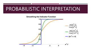
> 0

FITTING A LINEAR CLASSIFIER
 𝑓 𝑥; 𝑤 = 𝕀 𝑤𝑇
𝑥′
> 0
 How do we turn this into something continuous and
differentiable?
 We really want to replace the indicator function 𝕀 with a
smooth function indicating the probability of whether
𝑦 is 0 or 1, based on the value of 𝑤𝑇
𝑥′

PROBABILISTIC INTERPRETATION
 Interpreting 𝑤𝑇
𝑥′
 𝑤𝑇
𝑥′ large and positive
 ℙ 𝑦 = 0 ≪ ℙ[𝑦 = 1]
 𝑤𝑇
𝑥′ large and negative
 ℙ 𝑦 = 0 ≫ ℙ[𝑦 = 1]
 𝑤𝑇
𝑥′ small
 ℙ 𝑦 = 0 ≈ ℙ[𝑦 = 1]

 We therefore use the probability functions
 𝑝0 𝑥; 𝑤 = ℙ 𝑦 = 0 =
1
1+exp(𝑤𝑇𝑥′)
 𝑝1 𝑥; 𝑤 = ℙ 𝑦 = 1 =
exp(𝑤𝑇𝑥′)
1+exp(𝑤𝑇𝑥′)
 If 𝑤 = 𝑤 1
− 𝑤 0
as before, this is just
𝑝𝑘 𝑥; 𝑤 = ℙ 𝑦 = 𝑘 =
exp 𝑤 𝑘 𝑇
𝑥′
exp 𝑤 0 𝑇
𝑥′ +exp 𝑤 1 𝑇
𝑥′

 In the more general 𝑚-class case, we have
𝑝𝑘 𝑥; 𝐖 = ℙ 𝑦𝑘 = 1 =
exp 𝑤 𝑘 𝑇
𝑥′
𝑖=1
𝑚
exp 𝑤 𝑖 𝑇
𝑥′
 This is called the softmax activation and will be used
to define our loss function

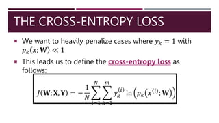
THE CROSS-ENTROPY LOSS
 We want to heavily penalize cases where 𝑦𝑘 = 1 with
𝑝𝑘 𝑥; 𝐖 ≪ 1
 This leads us to define the cross-entropy loss as
follows:
𝐽 𝐖; 𝐗, 𝐘 = −
1
𝑁
𝑖=1
𝑁
𝑘=1
𝑚
𝑦𝑘
𝑖
ln 𝑝𝑘 𝑥 𝑖
; 𝐖

MINIMIZING CROSS-ENTROPY
 As with mean-squared error, the cross-entropy loss is
convex and differentiable 
 That means that we can use gradient descent to
converge to a global minimum!
 This global minimum defines the best possible linear
classifier with respect to the cross-entropy loss and the
data set given

SUMMARY
 Basic process of constructing a machine learning model
 Choose an analytically well-behaved loss function that
represents some notion of error for your task
 Use gradient descent to choose model parameters that
minimize that loss function for your data set
 Examples: linear regression and mean squared error,
linear classification and cross-entropy

NEXT TIME
 Gradient of the cross-entropy loss
 Neural networks
 Backpropagation algorithm for gradient
descent

Machine learning introduction lecture notes

More Related Content

Similar to Machine learning introduction lecture notes (20)

Recently uploaded (20)

Machine learning introduction lecture notes

Editor's Notes