SlideShare a Scribd company logo
INDIAN INSTITUTE OF TECHNOLOGY ROORKEE
bala@cs.iitr.ac.in
https://faculty.iitr.ac.in/cs/bala/
CSN-382 (Lecture 10)
Dr. R. Balasubramanian
Professor
Department of Computer Science and Engineering
Mehta Family School of Data Science and Artificial Intelligence
Indian Institute of Technology Roorkee
Roorkee 247 667
Machine Learning
2
● Signal – all valid values for a variable (shows
between max and min values for x axis and y
axis). Represents a valid data.
● Noise – The spread of data points across the
best fit line. For a given value of x, there are
multiple values of y (some on line and some
around the line). This spread is due to random
factors.
● Signal to Noise Ratio – Variance of signal /
variance in noise.
● Greater the SNR the better the model will be.
X min X max
Signal
Y max
Y min
+
+
+
+
+
+
+
+
+
+ +
+
+
+
+
+
+
+
+
+
+
+
+
+
+
+
+
+
+
+
+
+
+
+
+
+
+
+
+ +
+
+
+ +
+
+
+
+
+
+
+
+
+
+
PCA (Signal to noise ratio)
3
● PCA can also be used to reduce
dimensions.
● Arrange all eigenvectors along with
corresponding eigenvalues in
descending order of eigenvalues.
● Plot a cumulative eigenvalue graph.
● Eigenvectors with insignificant
contribution to total eigenvalues
can be removed from analysis.
PCA for dimensionality reduction
4
Advantages Disadvantages
● Helps is reducing dimensions
● Correlated features are
removed
● Improves performance of an
algorithm
● Low noise sensitivity
● Assumes that feature set is correlated
● Sensitive to outliers
● High variance axis is treated as PC,
and low variance axes are treated as
noise
● Covariance matrix are difficult to be
evaluated in an accurate manner
Advantages and disadvantages
5
● Dimensionality reduction
● Improving signal to noise ratio
● Helps in removing correlation between variables
● To speed up the convergence of Neural networks
● Computer vision (Face recognition)
Applications of PCA
6
Feature Selection
► Instance based learning (kNN, last class)
 Not useful if the number of features is large.
► Feature Reduction
 Features contain information about the target.
► More features means better information or more information,
and better discriminative power or better classification power.
 But this may not be true always
7
Curse of Dimensionality
8
Curse of Dimensionality
► Irrelevant features
 In algorithm such as k nearest neighbor these irrelevant features
introduce noise and they fool the learning algorithm.
► Redundant features
 If you have a fixed number of training examples and redundant
features which do not contribute additional information they may
lead to degradation in performance of the learning algorithm.
► These irrelevant features and redundant features can confuse
learner, especially when you have limited training examples and
limited computational resources.
► Large number of features and limited training examples
 Overfitting
9
To overcome Curse of Dimensionality
► Feature Selection
► Feature Extraction
10
Feature Selection
► Given Set of initial features 𝐹 = {𝑥1, 𝑥2, 𝑥3, … , 𝑥𝑛}
► we can find 𝐹′ = {𝑥1′, 𝑥2′, 𝑥3′, … , 𝑥𝑚′}⊂ 𝐹
► We want to find a subset 𝐹′ of those features in 𝐹 so that it
optimizes certain criteria.
► How feature selection is differing from feature extraction.
► Feature selection in problems like hyperspectral imaging.
► From 𝑛 features set, we can have 2𝑛 possible feature subsets.
 Optimized algorithm in polynomial time
 Heuristic
 Greedy algorithm
 Randomized algorithm
11
Feature Subset Evaluation
► Unsupervised (Filter method)
► Supervised (Wrapper method)
12
Feature Selection Steps
► Feature Selection is an optimization problem:
► Step 1: Search the space of possible feature subsets.
► Step 2: Pick the subset that is optimal or near optimal w.r.t
some optimal function.
13
Feature Selection Steps
► Search Strategies
 Optimum
 Heuristic
 Randomized
► Evaluation Methods
 Filter methods
 Wrapper methods
14
Evaluating Feature Subset
► Supervised (Wrapper method)
 Train using selected subset
 Estimate error on validation dataset
► Unsupervised (Filter method)
 Look at input only
 Select the subset that has most input
15
Evaluation Strategies
16
Two different frameworks of feature
selection
► Find uncorrelated features in the reduced features
► Heuristic algorithms
 Forward Selection Algorithm
 Backward Selection Algorithm
► Forward Selection Algorithm
 Start with empty feature set and then you add features one by one
► Backward Selection Algorithm
 In backward search you start with the full feature set. Then you try
removing features from the features that you have.
17
Feature Selection
► Univariate (looks at each feature independently of others)
 Pearson correlation coefficient
 F-Score
 Chi-Square
 Signal to noise ratio
► Rank features by importance
► Ranking cut-off determined by user
► Univariate methods measure some type of correlation between
two random variables.
► The label 𝑦𝑖 and a fixed feature, 𝑥𝑖𝑗 for fixed 𝑗
18
Pearson correlation coefficient
► Please refer lecture 4 slides
19
● Signal – all valid values for a variable (shows
between max and min values for x axis and y
axis). Represents a valid data.
● Noise – The spread of data points across the
best fit line. For a given value of x, there are
multiple values of y (some on line and some
around the line). This spread is due to random
factors.
● Signal to Noise Ratio – Variance of signal /
variance in noise.
● Greater the SNR the better the model will be.
X min X max
Signal
Y max
Y min
+
+
+
+
+
+
+
+
+
+ +
+
+
+
+
+
+
+
+
+
+
+
+
+
+
+
+
+
+
+
+
+
+
+
+
+
+
+
+ +
+
+
+ +
+
+
+
+
+
+
+
+
+
+
Signal to noise ratio
20
Multivariate Feature Selection
► Multivariate (consider all features simultaneously).
► Consider the vector 𝑤 for any linear classifier.
► Classification of point 𝑥 is given by 𝑤𝑇𝑥 + 𝑤0.
► Small entries of 𝑤 will have little effect on dot product and hence
those features are less relevant.
► For example if 𝑤 = (10, 0.01, −9) then features 0 and 2 are
contributing more to a dot product than feature 1.
 A ranking of features given by this 𝑤 are 0,2 and 1.
► The 𝑤 can be obtained any of linear classifiers.
21
Multivariate Feature Selection
► A variant of this approach is called recursive feature elimination
 Compute 𝑤 on all features
 Remove features with smallest 𝑤𝑖
 Precompute 𝑤 on reduced data
 Goto step 2 if stopping criteria doesn’t meet.
22
Linear Discriminant Analysis
23
● Linear Discriminant Analysis is a supervised learning algorithm for
classification.
● Similar to PCA, it can be used for dimensionality reduction, by
projecting the input data to a linear subspace consisting of the
directions which maximize the separation between classes.
● It is a linear transformation technique.
● It can be used as a pre-processing stage for pattern-classification.
● The purpose of LDA is to lower the dimension space with a good
separability between the classes.
● It assumes that the features are normally distributed.
Linear Discriminant Analysis
24
Objective of LDA
25
● Fisher’s LDA aims to maximise
equation (1), maximize the distance
between means and minimize the
variance within classes
● Equation-1 can be rewritten with
two new terms:
○ Between class matrix (SB)
○ Within class matrix (SW)
Here, W is a unit vector
onto which the data points
are to be projected.
Objective of LDA
26
● Upon differentiating the equation
(2) w.r.t W and equating with 0, we
get a generalized eigenvalue-
eigenvector problem
○ SBW = vSwW
○ Sw
-1SBW = vW
■ Where v = eigenvalue
■ W = eigenvector
Objective of LDA
27
LDA
Matrix
● SB represents how precisely the data is
scattered across the classes
● Goal is to maximize SB. i.e. the distance
between the two classes should be
higher
Between
Class
Matrix(SB)
Step:2
● SW captures how precisely the data is
scattered within the class
● Goal is to minimize SW. i.e. the distance
between the elements of the class
should be minimum
Within
Class
Matrix(SW)
LDA Matrix
28
Linear Discriminant Analysis - Procedure
29
Thank You!

More Related Content

Similar to Machine Learning Notes for beginners ,Step by step (20)

PDF
Support Vector Machines ( SVM )
Mohammad Junaid Khan
 
PPTX
Machine learning and linear regression programming
Soumya Mukherjee
 
PPTX
cnn.pptx Convolutional neural network used for image classication
SakkaravarthiShanmug
 
PDF
Working with the data for Machine Learning
Mehwish690898
 
PDF
Beginners Guide to Non-Negative Matrix Factorization
Benjamin Bengfort
 
PPTX
Neural networks
HarshitGupta367
 
PPTX
Machine learning Module-2, 6th Semester Elective
MayuraD1
 
PPTX
svm-proyekt.pptx
ElinEliyev
 
PPT
INTRODUCTION TO ARTIFICIAL INTELLIGENCE.
SoumitraKundu4
 
PPTX
Ai saturdays presentation
Gurram Poorna Prudhvi
 
PPT
ai7.ppt
qwerty432737
 
PPT
ai7 (1) Artificial Neural Network Intro .ppt
AiniBasit
 
PDF
Machine Learning.pdf
BeyaNasr1
 
PPT
ai7.ppt
MrHacker61
 
PPT
Game theory.pdf textbooks content Artificical
webinartrainer
 
PPTX
Machine Learning Essentials Demystified part2 | Big Data Demystified
Omid Vahdaty
 
PPTX
Deeplearning for Computer Vision PPT with
naveenraghavendran10
 
PPT
Machine Learning Neural Networks Artificial
webinartrainer
 
PPT
Machine Learning Neural Networks Artificial Intelligence
webinartrainer
 
PPTX
Anomaly detection using deep one class classifier
홍배 김
 
Support Vector Machines ( SVM )
Mohammad Junaid Khan
 
Machine learning and linear regression programming
Soumya Mukherjee
 
cnn.pptx Convolutional neural network used for image classication
SakkaravarthiShanmug
 
Working with the data for Machine Learning
Mehwish690898
 
Beginners Guide to Non-Negative Matrix Factorization
Benjamin Bengfort
 
Neural networks
HarshitGupta367
 
Machine learning Module-2, 6th Semester Elective
MayuraD1
 
svm-proyekt.pptx
ElinEliyev
 
INTRODUCTION TO ARTIFICIAL INTELLIGENCE.
SoumitraKundu4
 
Ai saturdays presentation
Gurram Poorna Prudhvi
 
ai7.ppt
qwerty432737
 
ai7 (1) Artificial Neural Network Intro .ppt
AiniBasit
 
Machine Learning.pdf
BeyaNasr1
 
ai7.ppt
MrHacker61
 
Game theory.pdf textbooks content Artificical
webinartrainer
 
Machine Learning Essentials Demystified part2 | Big Data Demystified
Omid Vahdaty
 
Deeplearning for Computer Vision PPT with
naveenraghavendran10
 
Machine Learning Neural Networks Artificial
webinartrainer
 
Machine Learning Neural Networks Artificial Intelligence
webinartrainer
 
Anomaly detection using deep one class classifier
홍배 김
 

Recently uploaded (20)

PDF
Simplifying Document Processing with Docling for AI Applications.pdf
Tamanna
 
PDF
How to Connect Your On-Premises Site to AWS Using Site-to-Site VPN.pdf
Tamanna
 
PPTX
Exploring Multilingual Embeddings for Italian Semantic Search: A Pretrained a...
Sease
 
PDF
Avatar for apidays apidays PRO June 07, 2025 0 5 apidays Helsinki & North 2...
apidays
 
PDF
The European Business Wallet: Why It Matters and How It Powers the EUDI Ecosy...
Lal Chandran
 
PPT
tuberculosiship-2106031cyyfuftufufufivifviviv
AkshaiRam
 
PDF
OPPOTUS - Malaysias on Malaysia 1Q2025.pdf
Oppotus
 
PDF
Data Chunking Strategies for RAG in 2025.pdf
Tamanna
 
PDF
apidays Helsinki & North 2025 - Monetizing AI APIs: The New API Economy, Alla...
apidays
 
PPTX
SlideEgg_501298-Agentic AI.pptx agentic ai
530BYManoj
 
PPTX
Numbers of a nation: how we estimate population statistics | Accessible slides
Office for National Statistics
 
PDF
Driving Employee Engagement in a Hybrid World.pdf
Mia scott
 
PPTX
apidays Singapore 2025 - The Quest for the Greenest LLM , Jean Philippe Ehre...
apidays
 
PDF
Copia de Strategic Roadmap Infographics by Slidesgo.pptx (1).pdf
ssuserd4c6911
 
PDF
Context Engineering for AI Agents, approaches, memories.pdf
Tamanna
 
PDF
What does good look like - CRAP Brighton 8 July 2025
Jan Kierzyk
 
PDF
Merits and Demerits of DBMS over File System & 3-Tier Architecture in DBMS
MD RIZWAN MOLLA
 
PPTX
ER_Model_with_Diagrams_Presentation.pptx
dharaadhvaryu1992
 
PPTX
apidays Helsinki & North 2025 - APIs at Scale: Designing for Alignment, Trust...
apidays
 
PPTX
Module-5-Measures-of-Central-Tendency-Grouped-Data-1.pptx
lacsonjhoma0407
 
Simplifying Document Processing with Docling for AI Applications.pdf
Tamanna
 
How to Connect Your On-Premises Site to AWS Using Site-to-Site VPN.pdf
Tamanna
 
Exploring Multilingual Embeddings for Italian Semantic Search: A Pretrained a...
Sease
 
Avatar for apidays apidays PRO June 07, 2025 0 5 apidays Helsinki & North 2...
apidays
 
The European Business Wallet: Why It Matters and How It Powers the EUDI Ecosy...
Lal Chandran
 
tuberculosiship-2106031cyyfuftufufufivifviviv
AkshaiRam
 
OPPOTUS - Malaysias on Malaysia 1Q2025.pdf
Oppotus
 
Data Chunking Strategies for RAG in 2025.pdf
Tamanna
 
apidays Helsinki & North 2025 - Monetizing AI APIs: The New API Economy, Alla...
apidays
 
SlideEgg_501298-Agentic AI.pptx agentic ai
530BYManoj
 
Numbers of a nation: how we estimate population statistics | Accessible slides
Office for National Statistics
 
Driving Employee Engagement in a Hybrid World.pdf
Mia scott
 
apidays Singapore 2025 - The Quest for the Greenest LLM , Jean Philippe Ehre...
apidays
 
Copia de Strategic Roadmap Infographics by Slidesgo.pptx (1).pdf
ssuserd4c6911
 
Context Engineering for AI Agents, approaches, memories.pdf
Tamanna
 
What does good look like - CRAP Brighton 8 July 2025
Jan Kierzyk
 
Merits and Demerits of DBMS over File System & 3-Tier Architecture in DBMS
MD RIZWAN MOLLA
 
ER_Model_with_Diagrams_Presentation.pptx
dharaadhvaryu1992
 
apidays Helsinki & North 2025 - APIs at Scale: Designing for Alignment, Trust...
apidays
 
Module-5-Measures-of-Central-Tendency-Grouped-Data-1.pptx
lacsonjhoma0407
 
Ad

Machine Learning Notes for beginners ,Step by step

  • 1. INDIAN INSTITUTE OF TECHNOLOGY ROORKEE [email protected] https://faculty.iitr.ac.in/cs/bala/ CSN-382 (Lecture 10) Dr. R. Balasubramanian Professor Department of Computer Science and Engineering Mehta Family School of Data Science and Artificial Intelligence Indian Institute of Technology Roorkee Roorkee 247 667 Machine Learning
  • 2. 2 ● Signal – all valid values for a variable (shows between max and min values for x axis and y axis). Represents a valid data. ● Noise – The spread of data points across the best fit line. For a given value of x, there are multiple values of y (some on line and some around the line). This spread is due to random factors. ● Signal to Noise Ratio – Variance of signal / variance in noise. ● Greater the SNR the better the model will be. X min X max Signal Y max Y min + + + + + + + + + + + + + + + + + + + + + + + + + + + + + + + + + + + + + + + + + + + + + + + + + + + + + + PCA (Signal to noise ratio)
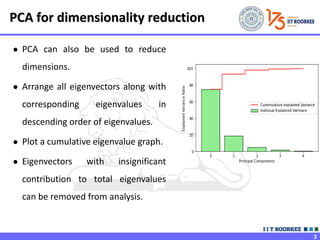
  • 3. 3 ● PCA can also be used to reduce dimensions. ● Arrange all eigenvectors along with corresponding eigenvalues in descending order of eigenvalues. ● Plot a cumulative eigenvalue graph. ● Eigenvectors with insignificant contribution to total eigenvalues can be removed from analysis. PCA for dimensionality reduction
  • 4. 4 Advantages Disadvantages ● Helps is reducing dimensions ● Correlated features are removed ● Improves performance of an algorithm ● Low noise sensitivity ● Assumes that feature set is correlated ● Sensitive to outliers ● High variance axis is treated as PC, and low variance axes are treated as noise ● Covariance matrix are difficult to be evaluated in an accurate manner Advantages and disadvantages
  • 5. 5 ● Dimensionality reduction ● Improving signal to noise ratio ● Helps in removing correlation between variables ● To speed up the convergence of Neural networks ● Computer vision (Face recognition) Applications of PCA
  • 6. 6 Feature Selection ► Instance based learning (kNN, last class)  Not useful if the number of features is large. ► Feature Reduction  Features contain information about the target. ► More features means better information or more information, and better discriminative power or better classification power.  But this may not be true always
  • 8. 8 Curse of Dimensionality ► Irrelevant features  In algorithm such as k nearest neighbor these irrelevant features introduce noise and they fool the learning algorithm. ► Redundant features  If you have a fixed number of training examples and redundant features which do not contribute additional information they may lead to degradation in performance of the learning algorithm. ► These irrelevant features and redundant features can confuse learner, especially when you have limited training examples and limited computational resources. ► Large number of features and limited training examples  Overfitting
  • 9. 9 To overcome Curse of Dimensionality ► Feature Selection ► Feature Extraction
  • 10. 10 Feature Selection ► Given Set of initial features 𝐹 = {𝑥1, 𝑥2, 𝑥3, … , 𝑥𝑛} ► we can find 𝐹′ = {𝑥1′, 𝑥2′, 𝑥3′, … , 𝑥𝑚′}⊂ 𝐹 ► We want to find a subset 𝐹′ of those features in 𝐹 so that it optimizes certain criteria. ► How feature selection is differing from feature extraction. ► Feature selection in problems like hyperspectral imaging. ► From 𝑛 features set, we can have 2𝑛 possible feature subsets.  Optimized algorithm in polynomial time  Heuristic  Greedy algorithm  Randomized algorithm
  • 11. 11 Feature Subset Evaluation ► Unsupervised (Filter method) ► Supervised (Wrapper method)
  • 12. 12 Feature Selection Steps ► Feature Selection is an optimization problem: ► Step 1: Search the space of possible feature subsets. ► Step 2: Pick the subset that is optimal or near optimal w.r.t some optimal function.
  • 13. 13 Feature Selection Steps ► Search Strategies  Optimum  Heuristic  Randomized ► Evaluation Methods  Filter methods  Wrapper methods
  • 14. 14 Evaluating Feature Subset ► Supervised (Wrapper method)  Train using selected subset  Estimate error on validation dataset ► Unsupervised (Filter method)  Look at input only  Select the subset that has most input
  • 16. 16 Two different frameworks of feature selection ► Find uncorrelated features in the reduced features ► Heuristic algorithms  Forward Selection Algorithm  Backward Selection Algorithm ► Forward Selection Algorithm  Start with empty feature set and then you add features one by one ► Backward Selection Algorithm  In backward search you start with the full feature set. Then you try removing features from the features that you have.
  • 17. 17 Feature Selection ► Univariate (looks at each feature independently of others)  Pearson correlation coefficient  F-Score  Chi-Square  Signal to noise ratio ► Rank features by importance ► Ranking cut-off determined by user ► Univariate methods measure some type of correlation between two random variables. ► The label 𝑦𝑖 and a fixed feature, 𝑥𝑖𝑗 for fixed 𝑗
  • 18. 18 Pearson correlation coefficient ► Please refer lecture 4 slides
  • 19. 19 ● Signal – all valid values for a variable (shows between max and min values for x axis and y axis). Represents a valid data. ● Noise – The spread of data points across the best fit line. For a given value of x, there are multiple values of y (some on line and some around the line). This spread is due to random factors. ● Signal to Noise Ratio – Variance of signal / variance in noise. ● Greater the SNR the better the model will be. X min X max Signal Y max Y min + + + + + + + + + + + + + + + + + + + + + + + + + + + + + + + + + + + + + + + + + + + + + + + + + + + + + + Signal to noise ratio
  • 20. 20 Multivariate Feature Selection ► Multivariate (consider all features simultaneously). ► Consider the vector 𝑤 for any linear classifier. ► Classification of point 𝑥 is given by 𝑤𝑇𝑥 + 𝑤0. ► Small entries of 𝑤 will have little effect on dot product and hence those features are less relevant. ► For example if 𝑤 = (10, 0.01, −9) then features 0 and 2 are contributing more to a dot product than feature 1.  A ranking of features given by this 𝑤 are 0,2 and 1. ► The 𝑤 can be obtained any of linear classifiers.
  • 21. 21 Multivariate Feature Selection ► A variant of this approach is called recursive feature elimination  Compute 𝑤 on all features  Remove features with smallest 𝑤𝑖  Precompute 𝑤 on reduced data  Goto step 2 if stopping criteria doesn’t meet.
  • 23. 23 ● Linear Discriminant Analysis is a supervised learning algorithm for classification. ● Similar to PCA, it can be used for dimensionality reduction, by projecting the input data to a linear subspace consisting of the directions which maximize the separation between classes. ● It is a linear transformation technique. ● It can be used as a pre-processing stage for pattern-classification. ● The purpose of LDA is to lower the dimension space with a good separability between the classes. ● It assumes that the features are normally distributed. Linear Discriminant Analysis
  • 25. 25 ● Fisher’s LDA aims to maximise equation (1), maximize the distance between means and minimize the variance within classes ● Equation-1 can be rewritten with two new terms: ○ Between class matrix (SB) ○ Within class matrix (SW) Here, W is a unit vector onto which the data points are to be projected. Objective of LDA
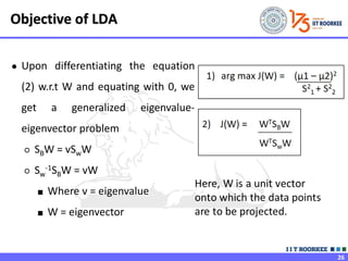
  • 26. 26 ● Upon differentiating the equation (2) w.r.t W and equating with 0, we get a generalized eigenvalue- eigenvector problem ○ SBW = vSwW ○ Sw -1SBW = vW ■ Where v = eigenvalue ■ W = eigenvector Objective of LDA
  • 27. 27 LDA Matrix ● SB represents how precisely the data is scattered across the classes ● Goal is to maximize SB. i.e. the distance between the two classes should be higher Between Class Matrix(SB) Step:2 ● SW captures how precisely the data is scattered within the class ● Goal is to minimize SW. i.e. the distance between the elements of the class should be minimum Within Class Matrix(SW) LDA Matrix