SlideShare a Scribd company logo
MATLAB TUTORIAL 4
By Norhan Abdalla
Outline:
■ Creating M-files
■ User Defined Functions
■ Solving Linear Equations
■ Symbolic Algebra
■ Calculus
CREATING M-FILES
MATLAB Environment
There are two ways to work with
MATLAB.
■ Command Window
• For small tasks or simple
calculations
• Will execute as soon as you press
Enter key
• Interactive ;as each command is
entered , a response is returned
■ M- files
• For large programs
• Known as m-files because of
their .m extension.
• Usually used when having user
defined functions.
Matlab M-files
■ To create M-files :
• File > New > Script
• Or use the shortcut ctrl +N
• Or from the toolbar , by clicking on the
icon called “New Script”
■ Running m- file:
• >>filename
• >>run filename
• >> run (‘filename’)
Saving your work
Using Diary
■ Another way of saving a segment
of code or calculations  using
the diary.
• >> diary on
• code
• >>diary off
• Or >> diary (‘filename’)
A file has
been
created
with the
variables
saved in
it.
Saving your work
■ After finishing code
instructions type the command
save .
■ It will create a file with
variables stored in it
• >> save filename
It saves the variables in
the work spaces and
allow to overwrite them
Cell Mode
■ Cell mode is a utility that allows you to divide M-
files into sections, or cells.
■ Each cell can be executed one at a time.
• From tab Cell >> Evaluate Current Cell
• Or ctrl + Enter
■ To divide M-file ,use
%% cell name
■ We can use the icons on the tool strip to evaluate a
single section.
■ To navigate between cells.
• From tab GO >> Go To
• Or ctrl + G
Dividing m-
file into cells
Formatting Results
• The format command controls
how tightly information is
spaced in the command
window.
• For example we took pi as an
number to represent different
formats
Command Display Example
format short 4 decimals 3.1416
format long 14 decimals 3.141592653589793
format short e 4 decimals in
scientific
3.1416e+000
format long e 14 decimals in
scientific
3.141592653589793e+000
format bank 2 decimals 3.14
format short eng 4 decimals in
engineering
3.1416e+000
format long eng 14 decimals in
engineering
3.14159265358979e+000
format + +, - , bank +
format rat Fractional form 355/113
format short g Matlab selects
the best format
3.1416
format long g Matlab selects
the best format
3.14159265358979
USER DEFINED
FUNCTIONS
User Defined Functions
■ Function: is a piece of
computer code that accepts an
input argument from the user
and provides output to the
program.
■ Functions allows us to program
efficiently.
• Creating functions is done
using M-files.
■ Function Definition:
1. The word ‘function’
2. A variable that defines the function
output
3. A function name
4. A variable used for the input argument
1 2 3 4
Defining a Function
■ To create a function , an M-file
must be created in the current
folder of the project and it
should have the same name as
the function .
Practice:
■ Create MATLAB functions to evaluate the following
mathematical functions.
• y(x) = 𝑥2
• y(x) = 𝑒 Τ
1
𝑥
• y(x) = sin(𝑥2
)
Hint:
To test your
function, you have
to call it from the
command window
Functions with Multiple Inputs and
Outputs
■ Multiple Inputs :
• For example ‘rem(x,y)’ takes two
inputs.
■ Similarly , a user defined function
could have multiple inputs.
• X and Y can be either scalars or
vectors.
■ Multiple Outputs:
• A function could return more
than one output. [output1 ,output2,…..]
If you call the
function without
specifying all the
three outputs ,
only the first one
is shown
Practice:
■ Assuming that the matrix dimensions agree, create and test
MATLAB functions to evaluate the following simplest
mathematical functions:
• 𝑧 𝑥, 𝑦 = 𝑥 + 𝑦
• 𝑧 𝑎, 𝑏, 𝑐 = 𝑎𝑏𝑐
• 𝑓 𝑥 = 5𝑥2
+ 2
• 𝑓 𝑥, 𝑦 = 𝑥 + 𝑦
• 𝑓 𝑥, 𝑦 = 𝑥𝑒𝑦
• 𝑓 𝑥 = 5𝑥2 + 2
Functions with No Inputs or
Outputs
■ Consider the following
function:
■ The square brackets indicates
an empty output function.
■ The parentheses indicates an
empty input function.
■ nargin() A function determines the
number of the input arguments in either a
user-defined function or a built-in
function.
■ nargout() A function determines the
number of the output arguments in either a
user-defined function or a built-in
function.
From the command window
-1
indicates
a
variable
of No
inputs
Local Variables
■ A local variable : is a variable
only accessed in its scope.
■ The variables used in functions
M-files are local variables.
■ Any variables defined within a
function exist only for that
function to use.
■ No local variables in a function
exist in the workspace.
g is not there
Global Variables
■ A global variable : is accessed
for all parts of a computer
program.
■ To use a global variable:
• Use the command ‘global var1’
■ It should be defined in the
command window or in a script
file
■ The global command alerts the
function to look in the
workspace for the value G.
■ This approach allows you to
change the value of G without
needing to redefine the
function in the M-file.
Accessing M-Files Code
■ The functions provided with
MATLAB are two types.
• Built in: its code is not
accessible.
• M-files stored in toolboxes
provided with the program.
■ We can see these M-files (or the
M-files we have written).
■ For example ,the sphere function
creates a three dimensional
shape.
■ Returns the contents of the
function you have defined earlier.
Try this:
Subfunctions:
■ More complicated functions can be
created together in a single file as
subfunctions.
■ Each MATLAB function M-file
has one primary function. The
name of the M-file must be the
same as the name of the primary
function name.
■ Subfunctions are added after
the primary function and can
have any variable name.
■ We use the ‘end’command to
indicate the end of each
individual function. This called
nesting.
Nesting : is when
the primary
function and other
subfunctions are
listed
sequentially.
SOLVING LINEAR
EQUATIONS
Polynomials
■ In MATLAB, a polynomial is
represented by a vector
■ To create a polynomial in
MATLAB, simply enter each
coefficient of the polynomial into
the vector in descending order.
■ For instance:
𝑥4
+ 3𝑥3
− 15𝑥2
− 2𝑥 + 9 , it can be
entered as a vector X = [ 1 ,3 ,-15 ,-2,9]
■ If it is missing any coefficients
, you must replace them by
entering zeros in the
appropriate place in the vector
• For example, 𝑥4
+ 1 it is saved
like this: Y = [ 1,0,0,0,1]
Polynomials
■ To find the value of the polynomial
y= 𝑥4
+ 1 at x =2
• Use the command:
• Z = polyval([1 0 0 0 1],2)
OR
• Z = polyval(y,2)
■ To extract the roots of a polynomial
such as : 𝑥2
− 5𝑥 + 6
• Use the command:
• Roots([1,-5 ,6])
System of Linear
Equations
■ Consider the following linear equations:
• 3x +2y –z = 10
• -x + 3y +2z = 5
• x –y – z = -1
• 𝐴 =
3 2 1
−1 3 2
1 −1 −1
𝑥
𝑦
𝑧
=
10
5
−1
1. Using the inverse:
System of Linear Equations
2. Using Gaussian elimination:
• Try this:
■ Consider the following equations:
• 3x +2y +5z = 22
• 4x + 5y -2z = 8
• x +y + z = 6
𝐴 =
3 2 5
4 5 −2
1 1 1
𝑥
𝑦
𝑧
=
22
8
6
System of Linear
Equations
3. Using the reverse row Echelon function:
■ Consider the following equations:
• 3x +2y -2z = 10
• -x + 3y +2z = 5
• x -y - z = -1
𝐴 =
3 2 1
−1 3 2
1 −1 −1
𝑥
𝑦
𝑧
=
10
5
−1
Solution of x ,y ,z
SYMBOLIC ALGEBRA
Symbolic Algebra
■ It is preferable to manipulate
the equations symbolically
before substituting values for
variables.
■ MATLAB ‘s symbolic algebra
capabilities allow you to
perform substituting ,
simplification , factorization,
..etc.
■ Creating symbolic variables:
• New variable:
• In the workspace:
or
They are in the
form of arrays
Practice:
■ You can declare multiple
symbolic at the same time.
■ Notice that:
■ Create the following symbolic variables, using
sym or syms command :
x, a ,b, c, d
■ Use the symbolic variables you created for the
following expressions:
• ex1 = 𝑎𝑥2
+ 𝑏𝑥 + 𝑐
• ex2 = sin(x)
• ex3 = sym (‘A𝑥3
+ 𝐵𝑥2
+ 𝐶𝑥 + 𝐹′)
• eq1= sym(‘ (x+1)^2=0 ’)
• eq2 = sym (‘ 𝐴𝑥2
= 1 ‘)
c and m are
not defined in
the workspace
Manipulating Symbolic
Expressions
■ MATLAB has a number of
functions designed to manipulate
symbolic variables.
• example:
■ poly2sym This function
requires a vector as input and
creates a symbolic variable.
■ sym2poly() This function
converts the symbolic variable to
a polynomial vector.
■ expands(s) Multiplies out all the portions of the
expression or equation.
■ factor(s) Factors the expression or the equation.
■ collect(s) Collects the terms.
■ simplify(s)  simplifies the equation or the expressions.
■ simple(s)  simplifies to the shortest representation of
the expression
■ numden(s)  Finds the numerator of an expression. This
function is not valid for equations.
■ [num,den] = numden(s)  Finds both the numerator and
the denominator of an expression.
Practice:
■ Create a variable y1= 𝑥2
− 1 * (𝑥 + 1)2
■ Create a variable y2= 𝑥2
− 1/(𝑥 + 1)2
■ Use the numden function to extract the numerator and
denominator from y1 and y2.
■ Use the factor, expand ,collect and simplify functions on y1
and y2.
Solving Expressions & Equations
■ Solve()  It can be used to determine the root of
expressions ,find numerical answers for a single variable,
to solve for an known symbolically.
■ MATLAB by default solves for x. If there is no x in the
expression , it finds the variable closest to x.
• To specify a variable to solve for:
The function
sets the
expression to
zero and solves
for roots
Solve for a
■ solve(S) Solves an expression with a single variable
■ solve(S) Solves an equation with more than one variable
■ solve (S, y) Solves an equation with more than one variable for a
specific variable.
■ [A,B,C] = solve(S1, S2, S3) Solves a system of equations and
assigns the solutions to the variables names.
Solving System of Equations
■ To solve a system of equations ,
define the equations as symbolic
variables , then use the ‘solve’
command
■ To solve For example:
■ You can also use this , but keep in
mind that the order of variable is
important
■ Remember that :
x,y,z are still symbolic variables.
■ To change the symbolic
variable to a numeric variable:
Use ‘double’
Practice:
■ Solve the following system of equations, use
all the techniques you learned so far:
5x+6y-3z=10
3x-3y+2z = 14
2x-4y-12= 24
Substitution
■ We can substitute inside the
function with either numbers or
variables.
■ We can define a vector of numbers through
substitution.
■ Note:
• If variables have been previously explicitly
defined symbolically , the quote is not
required.
You substitute y in the place of x
You substitute x with 3
Substituting by listing an array
to the variables in the equation
CALCULUS
Differentiation:
■ Use the command ‘diff(f)’
■ Consider the following:
■ diff(f ,’t’) Returns the
derivative of the expression f with
respect to the variable t
■ diff(f , n) Returns the nth
derivative.
■ diff(f, ‘t’, n) Returns the nth
derivative of the expression f with
respect to t.
Remember that the result is a
symbolic variable
Practice:
■ Find the first derivative:
• 𝑥2
+𝑥 + 1
• sin(x)
• ln(x)
■ Find the first partial derivative with respect to x:
• 𝑎𝑥2
+ 𝑏𝑥 + 𝑐
• tan 𝑥 + 𝑦
• 3𝑥 + 4𝑦 − 3𝑥𝑦
■ Find the second derivative with respect to y :
• 𝑦2
− 1
• 2𝑦 + 3𝑥2
Integration
■ To find the antiderivative,
use the command ‘int(f)’
■ int(f , ‘t’ )Returns the integral of f with
respect to variable t.
■ int(f , a ,b) Returns the integral of f
between the numeric values a , b.
■ int (f , ‘t’ , a ,b )  Returns the integral of f
with the respect to t between the numeric
values a, b .
• Note:
a , b can be either numbers or symbols
Practice:
■ Find the integral:
• 𝑥2
+𝑥 + 1
• sin(x)
• ln(x)
■ Integrate with respect to x:
• 𝑎𝑥2
+ 𝑏𝑥 + 𝑐
• tan 𝑥 + 𝑦
• 3𝑥 + 4𝑦 − 3𝑥𝑦
■ Integrate with respect to y :
• 𝑦2
− 1
• 2𝑦 + 3𝑥2
Try the same problems
with the limits ‫׬‬
0
5
𝑓
Differential Equations
𝑦 = 𝑒𝑡
𝑑𝑦
𝑑𝑡
= 𝑒𝑡
■ dsolve() requires the user to enter
the differential equation ,using the
symbol D to specify derivatives
with respect to the independent
variable.
• Hint:
Do not use the letter D in your variable
names in DE. The function will
interpret D as a derivative.
The default
independent
variable in
MATLAB is
t
With
initial
condition
Specifying the
independent
variable
Differential Equations
■ We can also use the ‘dsolve’
function to solve systems of
differential equations:
dsolve(‘ eq1 , eq2 , … cond 1 ,
cond 2,…’)
Symbolic
elements
in an array
To access the
component
of the array
Or

More Related Content

What's hot (20)

PDF
Matlab-Data types and operators
Luckshay Batra
 
PPTX
Basic matlab and matrix
Saidur Rahman
 
PPTX
Introduction to matlab
Khulna University
 
PPTX
Matlab Tutorial
Ahmad Siddiq
 
PPT
Basics of programming in matlab
AKANKSHA GUPTA
 
DOCX
MATLAB BASICS
butest
 
PDF
Matlab programming project
Assignmentpedia
 
PDF
Introduction to Matlab
Amr Rashed
 
PPTX
Basic operators in matlab
rishiteta
 
PPTX
Matlab for diploma students(1)
Retheesh Raj
 
PPSX
Matlab basic and image
Divyanshu Rasauria
 
PPT
Palm m3 chapter1b
Juan Pablo Fuentes Encinas
 
PPTX
Matlab introduction
Ameen San
 
PPTX
Introduction to matlab lecture 1 of 4
Randa Elanwar
 
PDF
Matlab from Beginner to Expert
smart-ideas
 
PPTX
C,C++ In Matlab
DataminingTools Inc
 
PDF
MATLAB Basics-Part1
Elaf A.Saeed
 
PDF
Introduction to MATLAB 1
Mohamed Gafar
 
PPT
Introduction to matlab
BilawalBaloch1
 
PPTX
Chapter 3.3
sotlsoc
 
Matlab-Data types and operators
Luckshay Batra
 
Basic matlab and matrix
Saidur Rahman
 
Introduction to matlab
Khulna University
 
Matlab Tutorial
Ahmad Siddiq
 
Basics of programming in matlab
AKANKSHA GUPTA
 
MATLAB BASICS
butest
 
Matlab programming project
Assignmentpedia
 
Introduction to Matlab
Amr Rashed
 
Basic operators in matlab
rishiteta
 
Matlab for diploma students(1)
Retheesh Raj
 
Matlab basic and image
Divyanshu Rasauria
 
Palm m3 chapter1b
Juan Pablo Fuentes Encinas
 
Matlab introduction
Ameen San
 
Introduction to matlab lecture 1 of 4
Randa Elanwar
 
Matlab from Beginner to Expert
smart-ideas
 
C,C++ In Matlab
DataminingTools Inc
 
MATLAB Basics-Part1
Elaf A.Saeed
 
Introduction to MATLAB 1
Mohamed Gafar
 
Introduction to matlab
BilawalBaloch1
 
Chapter 3.3
sotlsoc
 

Similar to Matlab tutorial 4 (20)

PPTX
introduction to matlab.pptx
Dr. Thippeswamy S.
 
PPT
MatlabIntro (1).ppt
AkashSingh728626
 
PDF
Matlab tutorial 3
Norhan Abdalla
 
PDF
Handout2.pdf
Shoukat13
 
PDF
A complete introduction on matlab and matlab's projects
Mukesh Kumar
 
PPT
Matlab Tutorial.ppt
RaviMuthamala1
 
PDF
Image processing
Pooya Sagharchiha
 
PPT
Introduction to Matlab.ppt
Ravibabu Kancharla
 
PDF
Scala qq
羽祈 張
 
PPT
MATLAB/SIMULINK for Engineering Applications day 2:Introduction to simulink
reddyprasad reddyvari
 
PDF
Dsp manual completed2
bilawalali74
 
PPTX
presentation.pptx
raghav415187
 
PPTX
1. Ch_1 SL_1_Intro to Matlab.pptx
MOHAMMAD SAYDUL ALAM
 
PPTX
An Introduction to MATLAB for beginners
Murshida ck
 
PPTX
Matlab ppt
chestialtaff
 
PDF
MATLAB_Practice_lect details about matlab3 (1).pdf
juhishrivastava25
 
PPTX
matlab presentation fro engninering students
SyedSadiq73
 
PDF
Section-6-User-Defined-Functions.pdf
johnkyllelumacang699
 
PDF
Matlab ch1 intro
Ragu Nathan
 
PDF
Matlab booklet
Sourabh Bhattacharya
 
introduction to matlab.pptx
Dr. Thippeswamy S.
 
MatlabIntro (1).ppt
AkashSingh728626
 
Matlab tutorial 3
Norhan Abdalla
 
Handout2.pdf
Shoukat13
 
A complete introduction on matlab and matlab's projects
Mukesh Kumar
 
Matlab Tutorial.ppt
RaviMuthamala1
 
Image processing
Pooya Sagharchiha
 
Introduction to Matlab.ppt
Ravibabu Kancharla
 
Scala qq
羽祈 張
 
MATLAB/SIMULINK for Engineering Applications day 2:Introduction to simulink
reddyprasad reddyvari
 
Dsp manual completed2
bilawalali74
 
presentation.pptx
raghav415187
 
1. Ch_1 SL_1_Intro to Matlab.pptx
MOHAMMAD SAYDUL ALAM
 
An Introduction to MATLAB for beginners
Murshida ck
 
Matlab ppt
chestialtaff
 
MATLAB_Practice_lect details about matlab3 (1).pdf
juhishrivastava25
 
matlab presentation fro engninering students
SyedSadiq73
 
Section-6-User-Defined-Functions.pdf
johnkyllelumacang699
 
Matlab ch1 intro
Ragu Nathan
 
Matlab booklet
Sourabh Bhattacharya
 
Ad

Recently uploaded (20)

PDF
ARC--BUILDING-UTILITIES-2-PART-2 (1).pdf
IzzyBaniquedBusto
 
PDF
monopile foundation seminar topic for civil engineering students
Ahina5
 
PPTX
UNIT DAA PPT cover all topics 2021 regulation
archu26
 
PPTX
Break Statement in Programming with 6 Real Examples
manojpoojary2004
 
PPTX
原版一样(Acadia毕业证书)加拿大阿卡迪亚大学毕业证办理方法
Taqyea
 
PPTX
Hashing Introduction , hash functions and techniques
sailajam21
 
PPTX
Pharmaceuticals and fine chemicals.pptxx
jaypa242004
 
PPTX
Green Building & Energy Conservation ppt
Sagar Sarangi
 
PDF
Statistical Data Analysis Using SPSS Software
shrikrishna kesharwani
 
PPTX
artificial intelligence applications in Geomatics
NawrasShatnawi1
 
PPTX
Structural Functiona theory this important for the theorist
cagumaydanny26
 
PPTX
MPMC_Module-2 xxxxxxxxxxxxxxxxxxxxx.pptx
ShivanshVaidya5
 
PPTX
265587293-NFPA 101 Life safety code-PPT-1.pptx
chandermwason
 
PPTX
Electron Beam Machining for Production Process
Rajshahi University of Engineering & Technology(RUET), Bangladesh
 
PPTX
Introduction to Neural Networks and Perceptron Learning Algorithm.pptx
Kayalvizhi A
 
PPTX
site survey architecture student B.arch.
sri02032006
 
PPTX
Presentation on Foundation Design for Civil Engineers.pptx
KamalKhan563106
 
PPTX
Innowell Capability B0425 - Commercial Buildings.pptx
regobertroza
 
PDF
PORTFOLIO Golam Kibria Khan — architect with a passion for thoughtful design...
MasumKhan59
 
PDF
Additional Information in midterm CPE024 (1).pdf
abolisojoy
 
ARC--BUILDING-UTILITIES-2-PART-2 (1).pdf
IzzyBaniquedBusto
 
monopile foundation seminar topic for civil engineering students
Ahina5
 
UNIT DAA PPT cover all topics 2021 regulation
archu26
 
Break Statement in Programming with 6 Real Examples
manojpoojary2004
 
原版一样(Acadia毕业证书)加拿大阿卡迪亚大学毕业证办理方法
Taqyea
 
Hashing Introduction , hash functions and techniques
sailajam21
 
Pharmaceuticals and fine chemicals.pptxx
jaypa242004
 
Green Building & Energy Conservation ppt
Sagar Sarangi
 
Statistical Data Analysis Using SPSS Software
shrikrishna kesharwani
 
artificial intelligence applications in Geomatics
NawrasShatnawi1
 
Structural Functiona theory this important for the theorist
cagumaydanny26
 
MPMC_Module-2 xxxxxxxxxxxxxxxxxxxxx.pptx
ShivanshVaidya5
 
265587293-NFPA 101 Life safety code-PPT-1.pptx
chandermwason
 
Electron Beam Machining for Production Process
Rajshahi University of Engineering & Technology(RUET), Bangladesh
 
Introduction to Neural Networks and Perceptron Learning Algorithm.pptx
Kayalvizhi A
 
site survey architecture student B.arch.
sri02032006
 
Presentation on Foundation Design for Civil Engineers.pptx
KamalKhan563106
 
Innowell Capability B0425 - Commercial Buildings.pptx
regobertroza
 
PORTFOLIO Golam Kibria Khan — architect with a passion for thoughtful design...
MasumKhan59
 
Additional Information in midterm CPE024 (1).pdf
abolisojoy
 
Ad

Matlab tutorial 4

  • 1. MATLAB TUTORIAL 4 By Norhan Abdalla
  • 2. Outline: ■ Creating M-files ■ User Defined Functions ■ Solving Linear Equations ■ Symbolic Algebra ■ Calculus
  • 4. MATLAB Environment There are two ways to work with MATLAB. ■ Command Window • For small tasks or simple calculations • Will execute as soon as you press Enter key • Interactive ;as each command is entered , a response is returned ■ M- files • For large programs • Known as m-files because of their .m extension. • Usually used when having user defined functions.
  • 5. Matlab M-files ■ To create M-files : • File > New > Script • Or use the shortcut ctrl +N • Or from the toolbar , by clicking on the icon called “New Script” ■ Running m- file: • >>filename • >>run filename • >> run (‘filename’)
  • 6. Saving your work Using Diary ■ Another way of saving a segment of code or calculations  using the diary. • >> diary on • code • >>diary off • Or >> diary (‘filename’) A file has been created with the variables saved in it.
  • 7. Saving your work ■ After finishing code instructions type the command save . ■ It will create a file with variables stored in it • >> save filename It saves the variables in the work spaces and allow to overwrite them
  • 8. Cell Mode ■ Cell mode is a utility that allows you to divide M- files into sections, or cells. ■ Each cell can be executed one at a time. • From tab Cell >> Evaluate Current Cell • Or ctrl + Enter ■ To divide M-file ,use %% cell name ■ We can use the icons on the tool strip to evaluate a single section. ■ To navigate between cells. • From tab GO >> Go To • Or ctrl + G Dividing m- file into cells
  • 9. Formatting Results • The format command controls how tightly information is spaced in the command window. • For example we took pi as an number to represent different formats Command Display Example format short 4 decimals 3.1416 format long 14 decimals 3.141592653589793 format short e 4 decimals in scientific 3.1416e+000 format long e 14 decimals in scientific 3.141592653589793e+000 format bank 2 decimals 3.14 format short eng 4 decimals in engineering 3.1416e+000 format long eng 14 decimals in engineering 3.14159265358979e+000 format + +, - , bank + format rat Fractional form 355/113 format short g Matlab selects the best format 3.1416 format long g Matlab selects the best format 3.14159265358979
  • 11. User Defined Functions ■ Function: is a piece of computer code that accepts an input argument from the user and provides output to the program. ■ Functions allows us to program efficiently. • Creating functions is done using M-files. ■ Function Definition: 1. The word ‘function’ 2. A variable that defines the function output 3. A function name 4. A variable used for the input argument 1 2 3 4
  • 12. Defining a Function ■ To create a function , an M-file must be created in the current folder of the project and it should have the same name as the function .
  • 13. Practice: ■ Create MATLAB functions to evaluate the following mathematical functions. • y(x) = 𝑥2 • y(x) = 𝑒 Τ 1 𝑥 • y(x) = sin(𝑥2 ) Hint: To test your function, you have to call it from the command window
  • 14. Functions with Multiple Inputs and Outputs ■ Multiple Inputs : • For example ‘rem(x,y)’ takes two inputs. ■ Similarly , a user defined function could have multiple inputs. • X and Y can be either scalars or vectors. ■ Multiple Outputs: • A function could return more than one output. [output1 ,output2,…..] If you call the function without specifying all the three outputs , only the first one is shown
  • 15. Practice: ■ Assuming that the matrix dimensions agree, create and test MATLAB functions to evaluate the following simplest mathematical functions: • 𝑧 𝑥, 𝑦 = 𝑥 + 𝑦 • 𝑧 𝑎, 𝑏, 𝑐 = 𝑎𝑏𝑐 • 𝑓 𝑥 = 5𝑥2 + 2 • 𝑓 𝑥, 𝑦 = 𝑥 + 𝑦 • 𝑓 𝑥, 𝑦 = 𝑥𝑒𝑦 • 𝑓 𝑥 = 5𝑥2 + 2
  • 16. Functions with No Inputs or Outputs ■ Consider the following function: ■ The square brackets indicates an empty output function. ■ The parentheses indicates an empty input function. ■ nargin() A function determines the number of the input arguments in either a user-defined function or a built-in function. ■ nargout() A function determines the number of the output arguments in either a user-defined function or a built-in function. From the command window -1 indicates a variable of No inputs
  • 17. Local Variables ■ A local variable : is a variable only accessed in its scope. ■ The variables used in functions M-files are local variables. ■ Any variables defined within a function exist only for that function to use. ■ No local variables in a function exist in the workspace. g is not there
  • 18. Global Variables ■ A global variable : is accessed for all parts of a computer program. ■ To use a global variable: • Use the command ‘global var1’ ■ It should be defined in the command window or in a script file ■ The global command alerts the function to look in the workspace for the value G. ■ This approach allows you to change the value of G without needing to redefine the function in the M-file.
  • 19. Accessing M-Files Code ■ The functions provided with MATLAB are two types. • Built in: its code is not accessible. • M-files stored in toolboxes provided with the program. ■ We can see these M-files (or the M-files we have written). ■ For example ,the sphere function creates a three dimensional shape. ■ Returns the contents of the function you have defined earlier. Try this:
  • 20. Subfunctions: ■ More complicated functions can be created together in a single file as subfunctions. ■ Each MATLAB function M-file has one primary function. The name of the M-file must be the same as the name of the primary function name. ■ Subfunctions are added after the primary function and can have any variable name. ■ We use the ‘end’command to indicate the end of each individual function. This called nesting. Nesting : is when the primary function and other subfunctions are listed sequentially.
  • 22. Polynomials ■ In MATLAB, a polynomial is represented by a vector ■ To create a polynomial in MATLAB, simply enter each coefficient of the polynomial into the vector in descending order. ■ For instance: 𝑥4 + 3𝑥3 − 15𝑥2 − 2𝑥 + 9 , it can be entered as a vector X = [ 1 ,3 ,-15 ,-2,9] ■ If it is missing any coefficients , you must replace them by entering zeros in the appropriate place in the vector • For example, 𝑥4 + 1 it is saved like this: Y = [ 1,0,0,0,1]
  • 23. Polynomials ■ To find the value of the polynomial y= 𝑥4 + 1 at x =2 • Use the command: • Z = polyval([1 0 0 0 1],2) OR • Z = polyval(y,2) ■ To extract the roots of a polynomial such as : 𝑥2 − 5𝑥 + 6 • Use the command: • Roots([1,-5 ,6])
  • 24. System of Linear Equations ■ Consider the following linear equations: • 3x +2y –z = 10 • -x + 3y +2z = 5 • x –y – z = -1 • 𝐴 = 3 2 1 −1 3 2 1 −1 −1 𝑥 𝑦 𝑧 = 10 5 −1 1. Using the inverse:
  • 25. System of Linear Equations 2. Using Gaussian elimination: • Try this: ■ Consider the following equations: • 3x +2y +5z = 22 • 4x + 5y -2z = 8 • x +y + z = 6 𝐴 = 3 2 5 4 5 −2 1 1 1 𝑥 𝑦 𝑧 = 22 8 6
  • 26. System of Linear Equations 3. Using the reverse row Echelon function: ■ Consider the following equations: • 3x +2y -2z = 10 • -x + 3y +2z = 5 • x -y - z = -1 𝐴 = 3 2 1 −1 3 2 1 −1 −1 𝑥 𝑦 𝑧 = 10 5 −1 Solution of x ,y ,z
  • 28. Symbolic Algebra ■ It is preferable to manipulate the equations symbolically before substituting values for variables. ■ MATLAB ‘s symbolic algebra capabilities allow you to perform substituting , simplification , factorization, ..etc. ■ Creating symbolic variables: • New variable: • In the workspace: or They are in the form of arrays
  • 29. Practice: ■ You can declare multiple symbolic at the same time. ■ Notice that: ■ Create the following symbolic variables, using sym or syms command : x, a ,b, c, d ■ Use the symbolic variables you created for the following expressions: • ex1 = 𝑎𝑥2 + 𝑏𝑥 + 𝑐 • ex2 = sin(x) • ex3 = sym (‘A𝑥3 + 𝐵𝑥2 + 𝐶𝑥 + 𝐹′) • eq1= sym(‘ (x+1)^2=0 ’) • eq2 = sym (‘ 𝐴𝑥2 = 1 ‘) c and m are not defined in the workspace
  • 30. Manipulating Symbolic Expressions ■ MATLAB has a number of functions designed to manipulate symbolic variables. • example: ■ poly2sym This function requires a vector as input and creates a symbolic variable. ■ sym2poly() This function converts the symbolic variable to a polynomial vector.
  • 31. ■ expands(s) Multiplies out all the portions of the expression or equation. ■ factor(s) Factors the expression or the equation. ■ collect(s) Collects the terms. ■ simplify(s)  simplifies the equation or the expressions. ■ simple(s)  simplifies to the shortest representation of the expression ■ numden(s)  Finds the numerator of an expression. This function is not valid for equations. ■ [num,den] = numden(s)  Finds both the numerator and the denominator of an expression.
  • 32. Practice: ■ Create a variable y1= 𝑥2 − 1 * (𝑥 + 1)2 ■ Create a variable y2= 𝑥2 − 1/(𝑥 + 1)2 ■ Use the numden function to extract the numerator and denominator from y1 and y2. ■ Use the factor, expand ,collect and simplify functions on y1 and y2.
  • 33. Solving Expressions & Equations ■ Solve()  It can be used to determine the root of expressions ,find numerical answers for a single variable, to solve for an known symbolically. ■ MATLAB by default solves for x. If there is no x in the expression , it finds the variable closest to x. • To specify a variable to solve for: The function sets the expression to zero and solves for roots Solve for a
  • 34. ■ solve(S) Solves an expression with a single variable ■ solve(S) Solves an equation with more than one variable ■ solve (S, y) Solves an equation with more than one variable for a specific variable. ■ [A,B,C] = solve(S1, S2, S3) Solves a system of equations and assigns the solutions to the variables names.
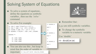
  • 35. Solving System of Equations ■ To solve a system of equations , define the equations as symbolic variables , then use the ‘solve’ command ■ To solve For example: ■ You can also use this , but keep in mind that the order of variable is important ■ Remember that : x,y,z are still symbolic variables. ■ To change the symbolic variable to a numeric variable: Use ‘double’
  • 36. Practice: ■ Solve the following system of equations, use all the techniques you learned so far: 5x+6y-3z=10 3x-3y+2z = 14 2x-4y-12= 24
  • 37. Substitution ■ We can substitute inside the function with either numbers or variables. ■ We can define a vector of numbers through substitution. ■ Note: • If variables have been previously explicitly defined symbolically , the quote is not required. You substitute y in the place of x You substitute x with 3 Substituting by listing an array to the variables in the equation
  • 39. Differentiation: ■ Use the command ‘diff(f)’ ■ Consider the following: ■ diff(f ,’t’) Returns the derivative of the expression f with respect to the variable t ■ diff(f , n) Returns the nth derivative. ■ diff(f, ‘t’, n) Returns the nth derivative of the expression f with respect to t. Remember that the result is a symbolic variable
  • 40. Practice: ■ Find the first derivative: • 𝑥2 +𝑥 + 1 • sin(x) • ln(x) ■ Find the first partial derivative with respect to x: • 𝑎𝑥2 + 𝑏𝑥 + 𝑐 • tan 𝑥 + 𝑦 • 3𝑥 + 4𝑦 − 3𝑥𝑦 ■ Find the second derivative with respect to y : • 𝑦2 − 1 • 2𝑦 + 3𝑥2
  • 41. Integration ■ To find the antiderivative, use the command ‘int(f)’ ■ int(f , ‘t’ )Returns the integral of f with respect to variable t. ■ int(f , a ,b) Returns the integral of f between the numeric values a , b. ■ int (f , ‘t’ , a ,b )  Returns the integral of f with the respect to t between the numeric values a, b . • Note: a , b can be either numbers or symbols
  • 42. Practice: ■ Find the integral: • 𝑥2 +𝑥 + 1 • sin(x) • ln(x) ■ Integrate with respect to x: • 𝑎𝑥2 + 𝑏𝑥 + 𝑐 • tan 𝑥 + 𝑦 • 3𝑥 + 4𝑦 − 3𝑥𝑦 ■ Integrate with respect to y : • 𝑦2 − 1 • 2𝑦 + 3𝑥2 Try the same problems with the limits ‫׬‬ 0 5 𝑓
  • 43. Differential Equations 𝑦 = 𝑒𝑡 𝑑𝑦 𝑑𝑡 = 𝑒𝑡 ■ dsolve() requires the user to enter the differential equation ,using the symbol D to specify derivatives with respect to the independent variable. • Hint: Do not use the letter D in your variable names in DE. The function will interpret D as a derivative. The default independent variable in MATLAB is t With initial condition Specifying the independent variable
  • 44. Differential Equations ■ We can also use the ‘dsolve’ function to solve systems of differential equations: dsolve(‘ eq1 , eq2 , … cond 1 , cond 2,…’) Symbolic elements in an array To access the component of the array Or