SlideShare a Scribd company logo
Practical 03-(Advance Features)
Creating spreadsheets with advance operations of Microsoft Excel
Objectives
 Be able to insert and create simple formulas.
 Be able to insert and create complex formulas.
 Be able to create and use functions.
 Be able to sort and filter the data.
 Be able to create and insert charts.
Tools
 MS Excel (Version: 2013, 2010 or 2007)
Keywords: Formula, Function, Sort, Filter. Duration: 03 hours
3 Introduction
3.1 Advance spreadsheet operations of MS Excel 2013
Besides the basic spreadsheet operations, MS Excel 2013 supports a wide range of advance
spreadsheet operations.
Few of the operations that are covered in this pracitcal are listed as:
 Formatting Cell Text
 Simple Formulas
 Complex Formulas
 Functions
 Sorting Data
 Filtering Data
 Inserting Charts
3.2 Formatting text and numbers
One of the most powerful tools in Excel is the ability to apply specific formatting for text and numbers.
Instead of displaying all cell content in exactly the same way, you can use formatting to change the
appearance of dates, times, decimals, percentages (%), currency ($), and much more.
3.2.1 To apply number formatting:
In our example, we'll change the number format for several cells to modify the way dates are
displayed.
1. Select the cells(s) you wish to modify.
2. Click the drop-down arrow next to the Number Format command on the Home tab. The Number
Formatting drop-down menu will appear.
3. Select the desired formatting option. In our example, we will change the formatting to Long Date.
4. The selected cells will change to the new formatting style. For some number formats, you can
then use the Increase Decimal and Decrease Decimal commands (below the Number Format
command) to change the number of decimal places that are displayed.
3.3 Simple Formulas
ation using formulas. Just like a calculator, Excel can add, subtract, multiply, and divide. In this lesson,
we'll show you how to use cell references to create simple formulas.
3.3.1 Mathematical operators
Excel uses standard operators for formulas, such as a plus sign for addition (+), a minus sign for
subtraction (-), an asterisk for multiplication (*), a forward slash for division (/), and a caret (^) for
exponents.
All formulas in Excel must begin with an equals sign (=). This is because the cell contains, or is equal
to, the formula and the value it calculates.
3.3.2 Understanding cell references
While you can create simple formulas in Excel manually (for example, =2+2 or =5*5), most of the time
you will use cell addresses to create a formula. This is known as making a cell reference. Using cell
references will ensure that your formulas are always accurate because you can change the value of
referenced cells without having to rewrite the formula.
By combining a mathematical operator with cell references, you can create a variety of simple
formulas in Excel. Formulas can also include a combination of cell references and numbers, as in the
examples below:
3.3.3 To create a formula:
In our example below, we'll use a simple formula and cell references to calculate a budget.
1. Select the cell that will contain the formula. In our example, we'll select cell B3.
2. Type the equals sign (=). Notice how it appears in both the cell and the formula bar.
3. Type the cell address of the cell you wish to reference first in the formula: cell B1 in our example.
A blue border will appear around the referenced cell.
4. Type the mathematical operator you wish to use. In our example, we'll type the addition sign (+).
5. Type the cell address of the cell you wish to reference second in the formula: cell B2 in our
example. A red border will appear around the referenced cell.
6. Press Enter on your keyboard. The formula will be calculated, and the value will be displayed in
the cell.
3.3.4 Modifying values with cell references
The true advantage of cell references is that they allow you to update data in your worksheet without
having to rewrite formulas. In the example below, we've modified the value of cell B1 from $1,200 to
$1,800. The formula in B3 will automatically recalculate and display the new value in cell B3.
3.3.5 To create a formula using the point-and-click method:
Rather than typing cell addresses manually, you can point and click on the cells you wish to include
in your formula. This method can save a lot of time and effort when creating formulas. In our example
below, we'll create a formula to calculate the cost of ordering several boxes of plastic silverware.
1. Select the cell that will contain the formula. In our example, we'll select cell D3.
2. Type the equals sign (=).
3. Select the cell you wish to reference first in the formula: cell B3 in our example. The cell address
will appear in the formula, and a dashed blue line will appear around the referenced cell.
4. Type the mathematical operator you wish to use. In our example, we'll type the multiplication
sign (*).
5. Select the cell you wish to reference second in the formula: cell C3 in our example. The cell
address will appear in the formula, and a dashed red line will appear around the referenced cell.
6. Press Enter on your keyboard. The formula will be calculated, and the value will be displayed in
the cell.
Formulas can also be copied to adjacent cells with the fill handle, which can save a lot of time and
effort if you need to perform the same calculation multiple times in a worksheet.
3.4 Complex Formulas
A simple formula is a mathematical expression with one operator, such as 7+9. A complex formula
has more than one mathematical operator, such as 5+2*8. When there is more than one operation in
a formula, the order of operations tells Excel which operation to calculate first. In order to use Excel
to calculate complex formulas, you will need to understand the order of operations.
3.4.1 Order of operations
Excel calculates formulas based on the following order of operations:
 Operations enclosed in parentheses
 Exponential calculations (3^2, for example)
 Multiplication and division, whichever comes first
 Addition and subtraction, whichever comes first
A mnemonic that can help you remember the order is PEMDAS, or Please Excuse My Dear Aunt Sally.
3.4.2 Creating complex formulas
In the example below, we will demonstrate how Excel solves a complex formula using the order of
operations. Here, we want to calculate the cost of sales tax for a catering invoice. To do this, we'll
write our formula as =(D2+D3)*0.075 in cell D4. This formula will add the prices of our items together
and then multiply that value by the 7.5% tax rate (which is written as 0.075) to calculate the cost of
sales tax.
Excel follows the order of operations and first adds the values inside the parentheses: (44.85+39.90)
= $84.75. Then, it multiplies that value by the tax rate: $84.75*0.075. The result will show that the
sales tax is $6.36.
It is especially important to enter complex formulas with the correct order of operations. Otherwise,
Excel will not calculate the results accurately. In our example, if the parentheses are not included, the
multiplication is calculated first and the result is incorrect. Parentheses are the best way to define
which calculations will be performed first in Excel.
3.4.3 To create a complex formula using the order of operations:
In our example below, we will use cell references along with numerical values to create a complex
formula that will calculate the total cost for a catering invoice. The formula will calculate the cost for
each menu item and then add those values together.
1. Select the cell that will contain the formula. In our example, we'll select cell C4.
2. Enter your formula. In our example, we'll type =B2*C2+B3*C3. This formula will follow the order
of operations, first performing the multiplication: 2.29*20 = 45.80 and 3.49*35 = 122.15. Then, it
will add those values together to calculate the total: 45.80+122.15.
3. Double-check your formula for accuracy, then press Enter on your keyboard. The formula will
calculate and display the result. In our example, the result shows that the total cost for the order
is $167.95.
3.5 Functions
A function is a predefined formula that performs calculations using specific values in a particular
order. Excel includes many common functions that can be useful for quickly finding the sum, average,
count, maximum value, and minimum value for a range of cells. In order to use functions correctly,
you'll need to understand the different parts of a function and how to create arguments to calculate
values and cell references.
3.5.1 The parts of a function
In order to work correctly, a function must be written a specific way, which is called the syntax. The
basic syntax for a function is an equals sign (=), the function name (SUM, for example), and one or
more arguments. Arguments contain the information you want to calculate. The function in the
example below would add the values of the cell range A1:A20.
3.5.2 Working with arguments
Arguments can refer to both individual cells and cell ranges and must be enclosed within
parentheses. You can include one argument or multiple arguments, depending on the syntax required
for the function.
For example, the function =AVERAGE(B1:B9) would calculate the average of the values in the cell
range B1:B9. This function contains only one argument.
Multiple arguments must be separated by a comma. For example, the function =SUM(A1:A3, C1:C2,
E2) will add the values of all the cells in the three arguments.
3.5.3 Creating a function
Excel has a variety of functions available. Here are some of the most common functions you'll use:
 SUM: This function adds all of the values of the cells in the argument.
 AVERAGE: This function determines the average of the values included in the argument. It
calculates the sum of the cells and then divides that value by the number of cells in the
argument.
 COUNT: This function counts the number of cells with numerical data in the argument. This
function is useful for quickly counting items in a cell range.
 MAX: This function determines the highest cell value included in the argument.
 MIN: This function determines the lowest cell value included in the argument.
3.5.3.1 To create a basic function:
In our example below, we'll create a basic function to calculate the average price per unit for a list of
recently ordered items using the AVERAGE function.
1. Select the cell that will contain the function. In our example, we'll select cell C11.
2. Type the equals sign (=) and enter the desired function name. You can also select the desired
function from the list of suggested functions that will appear below the cell as you type. In our
example, we'll type =AVERAGE.
3. Enter the cell range for the argument inside parentheses. In our example, we'll type (C3:C10).
This formula will add the values of cells C3:C10 and then divide that value by the total number of
cells in the range to determine the average.
4. Press Enter on your keyboard. The function will be calculated, and the result will appear in the
cell. In our example, the average price per unit of items ordered was $15.93.
3.5.3.2 To create a function using the AutoSum command:
The AutoSum command allows you to automatically insert the most common functions into your
formula, including SUM, AVERAGE, COUNT, MIN, and MAX. In our example below, we'll create a
function to calculate the total cost for a list of recently ordered items using the SUM function.
1. Select the cell that will contain the function. In our example, we'll select cell D12.
2. In the Editing group on the Home tab, locate and select the arrow next to the AutoSum command
and then choose the desired function from the drop-down menu. In our example, we'll select Sum.
3. The selected function will appear in the cell. If logically placed, the AutoSum command will
automatically select a cell range for the argument. In our example, cells D3:D11 were selected
automatically and their values will be added together to calculate the total cost. You can also
manually enter the desired cell range into the argument.
4. Press Enter on your keyboard. The function will be calculated, and the result will appear in the
cell. In our example, the sum of D3:D11 is $606.05.
The AutoSum command can also be accessed from the Formulas tab on the Ribbon.
3.5.4 The Function Library
While there are hundreds of functions in Excel, the ones you use most frequently will depend on the
type of data your workbooks contains. There is no need to learn every single function, but exploring
some of the different types of functions will be helpful as you create new projects. You can search for
functions by category, such as Financial, Logical, Text, Date & Time, and more from the Function
Library on the Formulas tab.
To access the Function Library, select the Formulas tab on the Ribbon. The Function Library will
appear.
3.5.4.1 To insert a function from the Function Library:
In our example below, we'll use a function to calculate the number of business days it took to receive
items after they were ordered. In our example, we'll use the dates in columns B and C to calculate the
delivery time in column D.
1. Select the cell that will contain the function. In our example, we'll select cell D3.
2. Click the Formulas tab on the Ribbon to access the Function Library.
3. From the Function Library group, select the desired function category. In our example, we'll
choose Date & Time.
4. Select the desired function from the drop-down menu. In our example, we'll select the
NETWORKDAYS function to count the number of business days between the ordered date and
received date.
5. The Function Arguments dialog box will appear. From here, you'll be able to enter or select the
cells that will make up the arguments in the function. In our example, we'll enter B3 in the
Start_date: field and C3 in the End_date: field.
6. When you're satisfied with the arguments, click OK.
7. The function will be calculated, and the result will appear in the cell. In our example, the result
shows that it took four business days to receive the order.
3.6 Sorting Data
As you add more content to a worksheet, organizing that information becomes especially important.
You can quickly reorganize a worksheet by sorting your data. For example, you could organize a list
of contact information by last name. Content can be sorted alphabetically, numerically, and in many
other ways.
3.6.1 Types of sorting
When sorting data, it's important to first decide if you would like the sort to apply to the entire
worksheet or just a cell range.
Sort sheet organizes all of the data in your worksheet by one column. Related information across
each row is kept together when the sort is applied. In the example below, the Contact Name column
(column A) has been sorted to display the names in alphabetical order.
Sort range sorts the data in a range of cells, which can be helpful when working with a sheet that
contains several tables. Sorting a range will not affect other content on the worksheet.
3.6.1.1 To sort a sheet:
In our example, we'll sort a T-shirt order form alphabetically by Last Name (column C).
1. Select a cell in the column you wish to sort by. In our example, we'll select cell C2.
2. Select the Data tab on the Ribbon, then click the Ascending command sort ascending to Sort A to
Z, or the Descending command sort ascending to Sort Z to A. In our example, we'll click the
Ascending command.
3. The worksheet will be sorted by the selected column. In our example, the worksheet is now
sorted by last name.
3.6.1.2 To sort a range:
In our example, we'll select a separate table in our T-shirt order form to sort the number of shirts
that were ordered on different dates.
1. Select the cell range you wish to sort. In our example, we'll select cell range A13:B17.
2. Select the Data tab on the Ribbon, then click the Sort command.
3. The Sort dialog box will appear. Choose the column you wish to sort by. In our example, we want
to sort the data by the number of T-shirt orders, so we'll select Orders.
4. Decide the sorting order (either ascending or descending). In our example, we'll use Smallest to
Largest.
5. Once you're satisfied with your selection, click OK.
6. The cell range will be sorted by the selected column. In our example, the Orders column will be
sorted from lowest to highest. Notice that the other content in the worksheet was not affected by
the sort.
3.7 Filtering Data
If your worksheet contains a lot of content, it can be difficult to find information quickly. Filters can
be used to narrow down the data in your worksheet, allowing you to view only the information you
need.
3.7.1 To filter data:
In our example, we'll apply a filter to an equipment log worksheet to display only the laptops and
projectors that are available for checkout.
In order for filtering to work correctly, your worksheet should include a header row, which is used
to identify the name of each column. In our example, our worksheet is organized into different
columns identified by the header cells in row 1: ID#, Type, Equipment Detail, and so on.
1. Select the Data tab, then click the Filter command.
2. A drop-down arrow will appear in the header cell for each column.
3. Click the drop-down arrow for the column you wish to filter. In our example, we will filter
column B to view only certain types of equipment.
4. The Filter menu will appear.
5. Uncheck the box next to Select All to quickly deselect all data.
6. Check the boxes next to the data you wish to filter, then click OK. In this example, we will check
Laptop and Tablet to view only those types of equipment.
7. The data will be filtered, temporarily hiding any content that doesn't match the criteria. In our
example, only laptops and tablets are visible.
3.7.2 To apply multiple filters:
Filters are cumulative, which means you can apply multiple filters to help narrow down your results.
In this example, we've already filtered our worksheet to show laptops and projectors, and we'd like
to narrow it down further to only show laptops and projectors that were checked out in August.
1. Click the drop-down arrow for the column you wish to filter. In this example, we will add a filter
to column D to view information by date.
2. The Filter menu will appear.
3. Check or uncheck the boxes depending on the data you wish to filter, then click OK. In our
example, we'll uncheck everything except for August.
4. The new filter will be applied. In our example, the worksheet is now filtered to show only laptops
and tablets that were checked out in August.
3.8 Charts
It can often be difficult to interpret Excel workbooks that contain a lot of data. Charts allow you to
illustrate your workbook data graphically, which makes it easy to visualize comparisons and trends.
3.8.1 Understanding charts
Excel has several different types of charts, allowing you to choose the one that best fits your data. In
order to use charts effectively, you'll need to understand how different charts are used.
In addition to chart types, you'll need to understand how to read a chart. Charts contain several
different elements, or parts, that can help you interpret the data.
3.8.2 To insert a chart:
1. Select the cells you want to chart, including the column titles and row labels. These cells will be
the source data for the chart. In our example, we'll select cells A1:F6.
2. From the Insert tab, click the desired Chart command. In our example, we'll select Column.
3. Choose the desired chart type from the drop-down menu.
4. The selected chart will be inserted in the worksheet.
EXERCISE
Create a spreadsheet in MS Excel that uses/contains the following:
 Formatting Cell Text
 Simple Formulas
 Complex Formulas
 Functions
 Data Sorting
 Data Filtering
 Charts

More Related Content

What's hot (20)

PPT
Excel Tutorial
Jayson Patalinghug
 
PDF
Algorithm and Programming (Introduction of Algorithms)
Adam Mukharil Bachtiar
 
PPT
Introduction to Excel
Najma Alam
 
PPT
Powerpoint class 3
Nicholas Charles
 
PPTX
Steps for c program execution
Rumman Ansari
 
PDF
Microsoft word exercises
Subeesh Up
 
PPT
Ms excel basic about Data, graph and pivot table
Alomgir Hossain
 
PPTX
Presentation
sindhu1801
 
PPTX
Libre Office Calc Lesson 4: Understanding Functions
Smart Chicago Collaborative
 
PPT
MS Excel 2nd
Adrian Apolinar Bulacan
 
DOCX
oxford computer books grade one chapter 1 to 3 question answer with exercise...
FaB6 Design
 
PPTX
Ms excel
Chirag Pahlajani
 
PPT
Number system
Sajib
 
PDF
Computer Programming
Syed Zaid Irshad
 
PPT
Excel IF, IFs.ppt
EdwinAdeolaOluwasina1
 
PPTX
Using Excel Functions
Gautam Gupta
 
PPTX
MS EXCEL lecture .pptx
cityhigh1
 
PPTX
Binary computing
samina khan
 
PPT
Ms excel ppt
Mukund Trivedi
 
PPTX
Number system
Suraj Bora
 
Excel Tutorial
Jayson Patalinghug
 
Algorithm and Programming (Introduction of Algorithms)
Adam Mukharil Bachtiar
 
Introduction to Excel
Najma Alam
 
Powerpoint class 3
Nicholas Charles
 
Steps for c program execution
Rumman Ansari
 
Microsoft word exercises
Subeesh Up
 
Ms excel basic about Data, graph and pivot table
Alomgir Hossain
 
Presentation
sindhu1801
 
Libre Office Calc Lesson 4: Understanding Functions
Smart Chicago Collaborative
 
oxford computer books grade one chapter 1 to 3 question answer with exercise...
FaB6 Design
 
Number system
Sajib
 
Computer Programming
Syed Zaid Irshad
 
Excel IF, IFs.ppt
EdwinAdeolaOluwasina1
 
Using Excel Functions
Gautam Gupta
 
MS EXCEL lecture .pptx
cityhigh1
 
Binary computing
samina khan
 
Ms excel ppt
Mukund Trivedi
 
Number system
Suraj Bora
 

Similar to Microsoft Excel Advanced Features (20)

PDF
Excel.fns frmls
rowenick
 
PPTX
CBN Advanced Excel Training Slide.pptx
EdwinAdeolaOluwasina1
 
PDF
Excel formulas-manual
srv1972
 
PPTX
Empowerment-Technologies-G11-W4-Q1-1.pptx
matthewesto
 
PDF
2. EXCEL BASICS.pdf IT course for medics
KAMAUFRANCISGATHUTHI
 
PDF
Excel 2003 tutorial 3
catacata1976
 
PDF
Simple formulas excel
Malika khalil
 
PDF
Excel (E-Module 2)
neha_gulati_ubs
 
PPT
Excelformulas
Heather Lambert
 
PPTX
Functions and formulas of ms excel
madhuparna bhowmik
 
PDF
Using microsoftexcelgj2 calculations
jeet121121
 
PDF
Using Microsoft Excel2 Calculations
Jack Frost
 
PPT
basic excels in information communication technology
JulieBinwag
 
PPT
22 Excel Basics
Buffalo Seminary
 
PDF
functionsandformulas-131221213835-phpapp01.pdf
FranzLawrenzDeTorres1
 
PPT
Excel 2007- Enter Formulas
Oklahoma Dept. Mental Health
 
PPT
22-excel-basics-15511.ppt
20ArnavKumar8F
 
PDF
Microsoft Excel 365 Formulas BarCharts QuickStudy 1st Edition Curtis Frye
ciuzajiram
 
PPT
03 ms excel
fosterstac
 
PDF
Tutorial Excel how to work with excel Tutorial Excel how to work with excel
HerySuhara1
 
Excel.fns frmls
rowenick
 
CBN Advanced Excel Training Slide.pptx
EdwinAdeolaOluwasina1
 
Excel formulas-manual
srv1972
 
Empowerment-Technologies-G11-W4-Q1-1.pptx
matthewesto
 
2. EXCEL BASICS.pdf IT course for medics
KAMAUFRANCISGATHUTHI
 
Excel 2003 tutorial 3
catacata1976
 
Simple formulas excel
Malika khalil
 
Excel (E-Module 2)
neha_gulati_ubs
 
Excelformulas
Heather Lambert
 
Functions and formulas of ms excel
madhuparna bhowmik
 
Using microsoftexcelgj2 calculations
jeet121121
 
Using Microsoft Excel2 Calculations
Jack Frost
 
basic excels in information communication technology
JulieBinwag
 
22 Excel Basics
Buffalo Seminary
 
functionsandformulas-131221213835-phpapp01.pdf
FranzLawrenzDeTorres1
 
Excel 2007- Enter Formulas
Oklahoma Dept. Mental Health
 
22-excel-basics-15511.ppt
20ArnavKumar8F
 
Microsoft Excel 365 Formulas BarCharts QuickStudy 1st Edition Curtis Frye
ciuzajiram
 
03 ms excel
fosterstac
 
Tutorial Excel how to work with excel Tutorial Excel how to work with excel
HerySuhara1
 
Ad

Recently uploaded (20)

PDF
Women's Health: Essential Tips for Every Stage.pdf
Iftikhar Ahmed
 
PPTX
SPINA BIFIDA: NURSING MANAGEMENT .pptx
PRADEEP ABOTHU
 
PDF
People & Earth's Ecosystem -Lesson 2: People & Population
marvinnbustamante1
 
PDF
BÀI TẬP BỔ TRỢ TIẾNG ANH 8 - GLOBAL SUCCESS - CẢ NĂM - NĂM 2024 (VOCABULARY, ...
Nguyen Thanh Tu Collection
 
PDF
community health nursing question paper 2.pdf
Prince kumar
 
PDF
The History of Phone Numbers in Stoke Newington by Billy Thomas
History of Stoke Newington
 
PPTX
I AM MALALA The Girl Who Stood Up for Education and was Shot by the Taliban...
Beena E S
 
PDF
Isharyanti-2025-Cross Language Communication in Indonesian Language
Neny Isharyanti
 
PDF
CONCURSO DE POESIA “POETUFAS – PASSOS SUAVES PELO VERSO.pdf
Colégio Santa Teresinha
 
PDF
The Constitution Review Committee (CRC) has released an updated schedule for ...
nservice241
 
PDF
SSHS-2025-PKLP_Quarter-1-Dr.-Kerby-Alvarez.pdf
AishahSangcopan1
 
PPTX
A PPT on Alfred Lord Tennyson's Ulysses.
Beena E S
 
PPTX
MENINGITIS: NURSING MANAGEMENT, BACTERIAL MENINGITIS, VIRAL MENINGITIS.pptx
PRADEEP ABOTHU
 
PPTX
grade 5 lesson matatag ENGLISH 5_Q1_PPT_WEEK4.pptx
SireQuinn
 
PDF
Reconstruct, Restore, Reimagine: New Perspectives on Stoke Newington’s Histor...
History of Stoke Newington
 
PPTX
Stereochemistry-Optical Isomerism in organic compoundsptx
Tarannum Nadaf-Mansuri
 
PDF
The-Ever-Evolving-World-of-Science (1).pdf/7TH CLASS CURIOSITY /1ST CHAPTER/B...
Sandeep Swamy
 
PDF
DIGESTION OF CARBOHYDRATES,PROTEINS,LIPIDS
raviralanaresh2
 
PPTX
2025 Winter SWAYAM NPTEL & A Student.pptx
Utsav Yagnik
 
PPTX
How to Convert an Opportunity into a Quotation in Odoo 18 CRM
Celine George
 
Women's Health: Essential Tips for Every Stage.pdf
Iftikhar Ahmed
 
SPINA BIFIDA: NURSING MANAGEMENT .pptx
PRADEEP ABOTHU
 
People & Earth's Ecosystem -Lesson 2: People & Population
marvinnbustamante1
 
BÀI TẬP BỔ TRỢ TIẾNG ANH 8 - GLOBAL SUCCESS - CẢ NĂM - NĂM 2024 (VOCABULARY, ...
Nguyen Thanh Tu Collection
 
community health nursing question paper 2.pdf
Prince kumar
 
The History of Phone Numbers in Stoke Newington by Billy Thomas
History of Stoke Newington
 
I AM MALALA The Girl Who Stood Up for Education and was Shot by the Taliban...
Beena E S
 
Isharyanti-2025-Cross Language Communication in Indonesian Language
Neny Isharyanti
 
CONCURSO DE POESIA “POETUFAS – PASSOS SUAVES PELO VERSO.pdf
Colégio Santa Teresinha
 
The Constitution Review Committee (CRC) has released an updated schedule for ...
nservice241
 
SSHS-2025-PKLP_Quarter-1-Dr.-Kerby-Alvarez.pdf
AishahSangcopan1
 
A PPT on Alfred Lord Tennyson's Ulysses.
Beena E S
 
MENINGITIS: NURSING MANAGEMENT, BACTERIAL MENINGITIS, VIRAL MENINGITIS.pptx
PRADEEP ABOTHU
 
grade 5 lesson matatag ENGLISH 5_Q1_PPT_WEEK4.pptx
SireQuinn
 
Reconstruct, Restore, Reimagine: New Perspectives on Stoke Newington’s Histor...
History of Stoke Newington
 
Stereochemistry-Optical Isomerism in organic compoundsptx
Tarannum Nadaf-Mansuri
 
The-Ever-Evolving-World-of-Science (1).pdf/7TH CLASS CURIOSITY /1ST CHAPTER/B...
Sandeep Swamy
 
DIGESTION OF CARBOHYDRATES,PROTEINS,LIPIDS
raviralanaresh2
 
2025 Winter SWAYAM NPTEL & A Student.pptx
Utsav Yagnik
 
How to Convert an Opportunity into a Quotation in Odoo 18 CRM
Celine George
 
Ad

Microsoft Excel Advanced Features

  • 1. Practical 03-(Advance Features) Creating spreadsheets with advance operations of Microsoft Excel Objectives  Be able to insert and create simple formulas.  Be able to insert and create complex formulas.  Be able to create and use functions.  Be able to sort and filter the data.  Be able to create and insert charts. Tools  MS Excel (Version: 2013, 2010 or 2007) Keywords: Formula, Function, Sort, Filter. Duration: 03 hours 3 Introduction 3.1 Advance spreadsheet operations of MS Excel 2013 Besides the basic spreadsheet operations, MS Excel 2013 supports a wide range of advance spreadsheet operations. Few of the operations that are covered in this pracitcal are listed as:  Formatting Cell Text  Simple Formulas  Complex Formulas  Functions  Sorting Data  Filtering Data  Inserting Charts
  • 2. 3.2 Formatting text and numbers One of the most powerful tools in Excel is the ability to apply specific formatting for text and numbers. Instead of displaying all cell content in exactly the same way, you can use formatting to change the appearance of dates, times, decimals, percentages (%), currency ($), and much more. 3.2.1 To apply number formatting: In our example, we'll change the number format for several cells to modify the way dates are displayed. 1. Select the cells(s) you wish to modify. 2. Click the drop-down arrow next to the Number Format command on the Home tab. The Number Formatting drop-down menu will appear. 3. Select the desired formatting option. In our example, we will change the formatting to Long Date.
  • 3. 4. The selected cells will change to the new formatting style. For some number formats, you can then use the Increase Decimal and Decrease Decimal commands (below the Number Format command) to change the number of decimal places that are displayed. 3.3 Simple Formulas ation using formulas. Just like a calculator, Excel can add, subtract, multiply, and divide. In this lesson, we'll show you how to use cell references to create simple formulas. 3.3.1 Mathematical operators Excel uses standard operators for formulas, such as a plus sign for addition (+), a minus sign for subtraction (-), an asterisk for multiplication (*), a forward slash for division (/), and a caret (^) for exponents.
  • 4. All formulas in Excel must begin with an equals sign (=). This is because the cell contains, or is equal to, the formula and the value it calculates. 3.3.2 Understanding cell references While you can create simple formulas in Excel manually (for example, =2+2 or =5*5), most of the time you will use cell addresses to create a formula. This is known as making a cell reference. Using cell references will ensure that your formulas are always accurate because you can change the value of referenced cells without having to rewrite the formula.
  • 5. By combining a mathematical operator with cell references, you can create a variety of simple formulas in Excel. Formulas can also include a combination of cell references and numbers, as in the examples below: 3.3.3 To create a formula: In our example below, we'll use a simple formula and cell references to calculate a budget. 1. Select the cell that will contain the formula. In our example, we'll select cell B3. 2. Type the equals sign (=). Notice how it appears in both the cell and the formula bar.
  • 6. 3. Type the cell address of the cell you wish to reference first in the formula: cell B1 in our example. A blue border will appear around the referenced cell. 4. Type the mathematical operator you wish to use. In our example, we'll type the addition sign (+). 5. Type the cell address of the cell you wish to reference second in the formula: cell B2 in our example. A red border will appear around the referenced cell. 6. Press Enter on your keyboard. The formula will be calculated, and the value will be displayed in the cell. 3.3.4 Modifying values with cell references The true advantage of cell references is that they allow you to update data in your worksheet without having to rewrite formulas. In the example below, we've modified the value of cell B1 from $1,200 to $1,800. The formula in B3 will automatically recalculate and display the new value in cell B3.
  • 7. 3.3.5 To create a formula using the point-and-click method: Rather than typing cell addresses manually, you can point and click on the cells you wish to include in your formula. This method can save a lot of time and effort when creating formulas. In our example below, we'll create a formula to calculate the cost of ordering several boxes of plastic silverware. 1. Select the cell that will contain the formula. In our example, we'll select cell D3. 2. Type the equals sign (=). 3. Select the cell you wish to reference first in the formula: cell B3 in our example. The cell address will appear in the formula, and a dashed blue line will appear around the referenced cell.
  • 8. 4. Type the mathematical operator you wish to use. In our example, we'll type the multiplication sign (*). 5. Select the cell you wish to reference second in the formula: cell C3 in our example. The cell address will appear in the formula, and a dashed red line will appear around the referenced cell. 6. Press Enter on your keyboard. The formula will be calculated, and the value will be displayed in the cell.
  • 9. Formulas can also be copied to adjacent cells with the fill handle, which can save a lot of time and effort if you need to perform the same calculation multiple times in a worksheet. 3.4 Complex Formulas A simple formula is a mathematical expression with one operator, such as 7+9. A complex formula has more than one mathematical operator, such as 5+2*8. When there is more than one operation in a formula, the order of operations tells Excel which operation to calculate first. In order to use Excel to calculate complex formulas, you will need to understand the order of operations. 3.4.1 Order of operations Excel calculates formulas based on the following order of operations:  Operations enclosed in parentheses  Exponential calculations (3^2, for example)  Multiplication and division, whichever comes first  Addition and subtraction, whichever comes first A mnemonic that can help you remember the order is PEMDAS, or Please Excuse My Dear Aunt Sally.
  • 10. 3.4.2 Creating complex formulas In the example below, we will demonstrate how Excel solves a complex formula using the order of operations. Here, we want to calculate the cost of sales tax for a catering invoice. To do this, we'll write our formula as =(D2+D3)*0.075 in cell D4. This formula will add the prices of our items together and then multiply that value by the 7.5% tax rate (which is written as 0.075) to calculate the cost of sales tax. Excel follows the order of operations and first adds the values inside the parentheses: (44.85+39.90) = $84.75. Then, it multiplies that value by the tax rate: $84.75*0.075. The result will show that the sales tax is $6.36. It is especially important to enter complex formulas with the correct order of operations. Otherwise, Excel will not calculate the results accurately. In our example, if the parentheses are not included, the multiplication is calculated first and the result is incorrect. Parentheses are the best way to define which calculations will be performed first in Excel.
  • 11. 3.4.3 To create a complex formula using the order of operations: In our example below, we will use cell references along with numerical values to create a complex formula that will calculate the total cost for a catering invoice. The formula will calculate the cost for each menu item and then add those values together. 1. Select the cell that will contain the formula. In our example, we'll select cell C4. 2. Enter your formula. In our example, we'll type =B2*C2+B3*C3. This formula will follow the order of operations, first performing the multiplication: 2.29*20 = 45.80 and 3.49*35 = 122.15. Then, it will add those values together to calculate the total: 45.80+122.15. 3. Double-check your formula for accuracy, then press Enter on your keyboard. The formula will calculate and display the result. In our example, the result shows that the total cost for the order is $167.95.
  • 12. 3.5 Functions A function is a predefined formula that performs calculations using specific values in a particular order. Excel includes many common functions that can be useful for quickly finding the sum, average, count, maximum value, and minimum value for a range of cells. In order to use functions correctly, you'll need to understand the different parts of a function and how to create arguments to calculate values and cell references. 3.5.1 The parts of a function In order to work correctly, a function must be written a specific way, which is called the syntax. The basic syntax for a function is an equals sign (=), the function name (SUM, for example), and one or more arguments. Arguments contain the information you want to calculate. The function in the example below would add the values of the cell range A1:A20. 3.5.2 Working with arguments Arguments can refer to both individual cells and cell ranges and must be enclosed within parentheses. You can include one argument or multiple arguments, depending on the syntax required for the function. For example, the function =AVERAGE(B1:B9) would calculate the average of the values in the cell range B1:B9. This function contains only one argument.
  • 13. Multiple arguments must be separated by a comma. For example, the function =SUM(A1:A3, C1:C2, E2) will add the values of all the cells in the three arguments. 3.5.3 Creating a function Excel has a variety of functions available. Here are some of the most common functions you'll use:  SUM: This function adds all of the values of the cells in the argument.  AVERAGE: This function determines the average of the values included in the argument. It calculates the sum of the cells and then divides that value by the number of cells in the argument.  COUNT: This function counts the number of cells with numerical data in the argument. This function is useful for quickly counting items in a cell range.  MAX: This function determines the highest cell value included in the argument.  MIN: This function determines the lowest cell value included in the argument. 3.5.3.1 To create a basic function: In our example below, we'll create a basic function to calculate the average price per unit for a list of recently ordered items using the AVERAGE function. 1. Select the cell that will contain the function. In our example, we'll select cell C11.
  • 14. 2. Type the equals sign (=) and enter the desired function name. You can also select the desired function from the list of suggested functions that will appear below the cell as you type. In our example, we'll type =AVERAGE. 3. Enter the cell range for the argument inside parentheses. In our example, we'll type (C3:C10). This formula will add the values of cells C3:C10 and then divide that value by the total number of cells in the range to determine the average.
  • 15. 4. Press Enter on your keyboard. The function will be calculated, and the result will appear in the cell. In our example, the average price per unit of items ordered was $15.93. 3.5.3.2 To create a function using the AutoSum command: The AutoSum command allows you to automatically insert the most common functions into your formula, including SUM, AVERAGE, COUNT, MIN, and MAX. In our example below, we'll create a function to calculate the total cost for a list of recently ordered items using the SUM function. 1. Select the cell that will contain the function. In our example, we'll select cell D12. 2. In the Editing group on the Home tab, locate and select the arrow next to the AutoSum command and then choose the desired function from the drop-down menu. In our example, we'll select Sum.
  • 16. 3. The selected function will appear in the cell. If logically placed, the AutoSum command will automatically select a cell range for the argument. In our example, cells D3:D11 were selected automatically and their values will be added together to calculate the total cost. You can also manually enter the desired cell range into the argument. 4. Press Enter on your keyboard. The function will be calculated, and the result will appear in the cell. In our example, the sum of D3:D11 is $606.05.
  • 17. The AutoSum command can also be accessed from the Formulas tab on the Ribbon. 3.5.4 The Function Library While there are hundreds of functions in Excel, the ones you use most frequently will depend on the type of data your workbooks contains. There is no need to learn every single function, but exploring some of the different types of functions will be helpful as you create new projects. You can search for functions by category, such as Financial, Logical, Text, Date & Time, and more from the Function Library on the Formulas tab. To access the Function Library, select the Formulas tab on the Ribbon. The Function Library will appear. 3.5.4.1 To insert a function from the Function Library: In our example below, we'll use a function to calculate the number of business days it took to receive items after they were ordered. In our example, we'll use the dates in columns B and C to calculate the delivery time in column D.
  • 18. 1. Select the cell that will contain the function. In our example, we'll select cell D3. 2. Click the Formulas tab on the Ribbon to access the Function Library. 3. From the Function Library group, select the desired function category. In our example, we'll choose Date & Time. 4. Select the desired function from the drop-down menu. In our example, we'll select the NETWORKDAYS function to count the number of business days between the ordered date and received date.
  • 19. 5. The Function Arguments dialog box will appear. From here, you'll be able to enter or select the cells that will make up the arguments in the function. In our example, we'll enter B3 in the Start_date: field and C3 in the End_date: field. 6. When you're satisfied with the arguments, click OK. 7. The function will be calculated, and the result will appear in the cell. In our example, the result shows that it took four business days to receive the order. 3.6 Sorting Data As you add more content to a worksheet, organizing that information becomes especially important. You can quickly reorganize a worksheet by sorting your data. For example, you could organize a list of contact information by last name. Content can be sorted alphabetically, numerically, and in many other ways. 3.6.1 Types of sorting When sorting data, it's important to first decide if you would like the sort to apply to the entire worksheet or just a cell range.
  • 20. Sort sheet organizes all of the data in your worksheet by one column. Related information across each row is kept together when the sort is applied. In the example below, the Contact Name column (column A) has been sorted to display the names in alphabetical order. Sort range sorts the data in a range of cells, which can be helpful when working with a sheet that contains several tables. Sorting a range will not affect other content on the worksheet.
  • 21. 3.6.1.1 To sort a sheet: In our example, we'll sort a T-shirt order form alphabetically by Last Name (column C). 1. Select a cell in the column you wish to sort by. In our example, we'll select cell C2. 2. Select the Data tab on the Ribbon, then click the Ascending command sort ascending to Sort A to Z, or the Descending command sort ascending to Sort Z to A. In our example, we'll click the Ascending command. 3. The worksheet will be sorted by the selected column. In our example, the worksheet is now sorted by last name.
  • 22. 3.6.1.2 To sort a range: In our example, we'll select a separate table in our T-shirt order form to sort the number of shirts that were ordered on different dates. 1. Select the cell range you wish to sort. In our example, we'll select cell range A13:B17. 2. Select the Data tab on the Ribbon, then click the Sort command. 3. The Sort dialog box will appear. Choose the column you wish to sort by. In our example, we want to sort the data by the number of T-shirt orders, so we'll select Orders.
  • 23. 4. Decide the sorting order (either ascending or descending). In our example, we'll use Smallest to Largest. 5. Once you're satisfied with your selection, click OK. 6. The cell range will be sorted by the selected column. In our example, the Orders column will be sorted from lowest to highest. Notice that the other content in the worksheet was not affected by the sort. 3.7 Filtering Data If your worksheet contains a lot of content, it can be difficult to find information quickly. Filters can be used to narrow down the data in your worksheet, allowing you to view only the information you need.
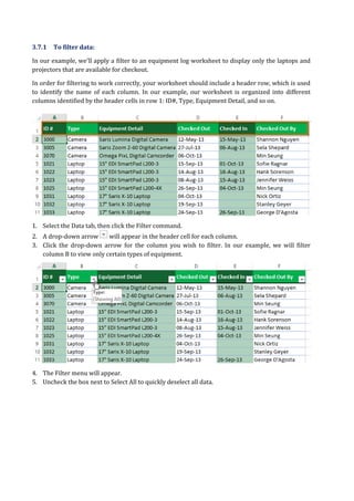
  • 24. 3.7.1 To filter data: In our example, we'll apply a filter to an equipment log worksheet to display only the laptops and projectors that are available for checkout. In order for filtering to work correctly, your worksheet should include a header row, which is used to identify the name of each column. In our example, our worksheet is organized into different columns identified by the header cells in row 1: ID#, Type, Equipment Detail, and so on. 1. Select the Data tab, then click the Filter command. 2. A drop-down arrow will appear in the header cell for each column. 3. Click the drop-down arrow for the column you wish to filter. In our example, we will filter column B to view only certain types of equipment. 4. The Filter menu will appear. 5. Uncheck the box next to Select All to quickly deselect all data.
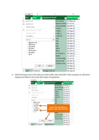
  • 25. 6. Check the boxes next to the data you wish to filter, then click OK. In this example, we will check Laptop and Tablet to view only those types of equipment.
  • 26. 7. The data will be filtered, temporarily hiding any content that doesn't match the criteria. In our example, only laptops and tablets are visible. 3.7.2 To apply multiple filters: Filters are cumulative, which means you can apply multiple filters to help narrow down your results. In this example, we've already filtered our worksheet to show laptops and projectors, and we'd like to narrow it down further to only show laptops and projectors that were checked out in August. 1. Click the drop-down arrow for the column you wish to filter. In this example, we will add a filter to column D to view information by date. 2. The Filter menu will appear. 3. Check or uncheck the boxes depending on the data you wish to filter, then click OK. In our example, we'll uncheck everything except for August.
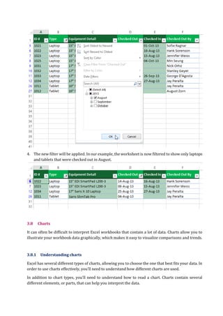
  • 27. 4. The new filter will be applied. In our example, the worksheet is now filtered to show only laptops and tablets that were checked out in August. 3.8 Charts It can often be difficult to interpret Excel workbooks that contain a lot of data. Charts allow you to illustrate your workbook data graphically, which makes it easy to visualize comparisons and trends. 3.8.1 Understanding charts Excel has several different types of charts, allowing you to choose the one that best fits your data. In order to use charts effectively, you'll need to understand how different charts are used. In addition to chart types, you'll need to understand how to read a chart. Charts contain several different elements, or parts, that can help you interpret the data.
  • 28. 3.8.2 To insert a chart: 1. Select the cells you want to chart, including the column titles and row labels. These cells will be the source data for the chart. In our example, we'll select cells A1:F6. 2. From the Insert tab, click the desired Chart command. In our example, we'll select Column. 3. Choose the desired chart type from the drop-down menu.
  • 29. 4. The selected chart will be inserted in the worksheet.
  • 30. EXERCISE Create a spreadsheet in MS Excel that uses/contains the following:  Formatting Cell Text  Simple Formulas  Complex Formulas  Functions  Data Sorting  Data Filtering  Charts