Minimum Spanning Trees Artificial Intelligence

DESIGN AND ANALYSIS OF
ALGORITHM
(CS206)
MODULE-4
GREEDY METHOD

Greedy and other Design Approaches
Introduction to Greedy using-
- fractional knapsack problem
- Huffman Code
Minimum Spanning Tree-
- Prim’s and Kruskal’s algorithms
Single Source Shortest Paths-
- Dijkstra’s and Bellman-Ford algorithms
Introduction to Backtracking using
- N-Queens problem,
Introduction to Branch and Bound using
- Assignment Problem or Traveling Salesman Problem.

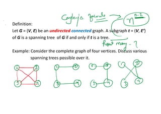
Definition:
Let G = (V, E) be an undirected connected graph. A subgraph t = (V, E’)
of G is a spanning tree of G if and only if t is a tree.
Example: Consider the complete graph of four vertices. Discuss various
spanning trees possible over it.

Applications:
• They can be used to obtain an independent set of circuit equations
for an electric network.
• Another application of spanning trees arises from the property that a
spanning tree is a minimal subgraph G’ of G such that V(G’) = V(G)
and G’ is connected.
Any connected graph with n vertices must have at least n-1 edges and
all connected graphs with n-1 edges are trees. If the nodes of G
represent cities and the edges represent possible communication link
connecting two cities, then the minimum number of links needed to
connect the n cities is n-1. The spanning trees of G represent all
feasible choices.

Approach: Build the spanning tree edge by edge.
Question: How to choose the next edge?
or
What is the optimization criterion?
Solution: Choose an edge that results in a minimum increase in the
sum of the costs of the edges so far included.
There are two possible ways to interpret this criterion.

Interpretation (01):
The set of edges so far selected form a tree.
Thus, if A = set of edges selected so far, then A forms a tree.
The next edge (u, v) to be included in A should have property that
A U {(u, v)} is also a tree.
Question: Show that this selection criterion results in a minimum cost
spanning tree.
The corresponding approach is known as PRIM’S algorithm.

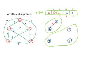
Approach-
The algorithm starts with a tree that includes only a minimum cost
edge of graph G.
Then, edges are added to this tree one by one.
The next edge (i, j) to be added is such that:
i is already in partial spanning tree T
j is not in the tree T.
Cost(i, j) = minimum among all the edges (k, l) such that:
k is in the tree T and
l is not in the tree T.
Key to this approach is to determine edge(I, j) efficiently.

Algorithm PRIM (C, n)
{
// Let G is a connected undirected graph, C is the cost adjacency matrix.
// n is the number of vertices in G, T is the minimum weight spanning tree.
for (i=1; I ≤ n; i++)
visited[i] = 0; // Initialize all vertices as unvisited
u = 1; // Consider vertex 1 as starting
visited[u] = 1;
T = ɸ // initially
while (there is still unchosen vertex)
{
let <u, v> be the lightest edge between any chosen u and any unchosen v;
visited[v] = 1;
T = Union (T, <u, v>); // add edge to spanning tree
}
}

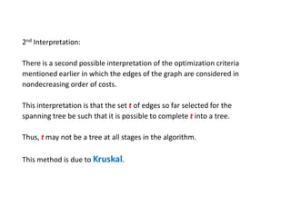
2nd Interpretation:
There is a second possible interpretation of the optimization criteria
mentioned earlier in which the edges of the graph are considered in
nondecreasing order of costs.
This interpretation is that the set t of edges so far selected for the
spanning tree be such that it is possible to complete t into a tree.
Thus, t may not be a tree at all stages in the algorithm.
This method is due to Kruskal.

// Early form of minimum-cost spanning tree algorithm due to Kruskal
Algorithm: Kruskal
1. t = ɸ;
2. while ((t has less than n-1 edges) and (E ≠ ɸ)) do
3. {
4. Choose an edge (v, w) from E of lowest cost;
5. Delete (v, w) from E;
6. if (v, w) does not create a cycle in t then add (v, w) to t;
7. else discard (v, w);
8. }

Introduction:
Two sets Si and Sj, i!=j, are said to be pairwise disjoint if there is no
element that is in both Si and Sj.
Example:
Given n = 10, the elements can be partitioned into three disjoint sets,
S1 = {1, 7, 8, 9}
S2 = {2, 5, 10} and
S3 = {3, 4, 6}

S1 = {1, 7, 8, 9}
S2 = {2, 5, 10} and
S3 = {3, 4, 6}

The operations we wish to perform on these sets are:
(1) Disjoint set union: If Si and Sj are two disjoint sets, then their union
Si U Si = all elements x such that x is in Si or Sj.
In this process, the sets Si and Sj are replaced by Si U Sj in the
collection of sets.
(2) Find(i): Given the element i, find the set containing i.
Thus, 4 is in set S3, and 9 is in set S1.

How to implement Find (i) ?
Algorithm SimpleFind (i)
{
while (P[i] >= 0)
{
i= P[i];
}
return (i);
}

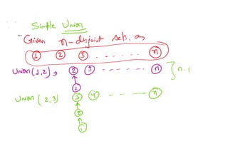
How to implement operation Simple Union (i, j) ?
We have two trees with roots i and j.
Convention: First tree becomes a subtree of the second.
The statement P[i] = j, accomplishes the Union.

Improved Union algorithm:
Definition: [Weighting rule for Union(i, j)] If the number of nodes in the
tree with root i is less than the number in the tree with root
j, then make j the parent of i; otherwise make i the parent
of j.

To implement the weighting rule, we need to know how many nodes
there are in every tree.
 To do this easily, we maintain a count field in the root of every tree.
 If i is a root node, then count[i] equals the number of nodes in that
tree.

Algorithm WeightedUnion (i, j)
// Union sets with root i and j, i!= j, using the weighting rule.
// p[i] = -count[i] and p[j] = -count[j].
{
temp = p[i] + p[j];
if (p[i] > p[j]) then
{
// i has fewer nodes.
p[i] = j; p[j] = temp;
}
else
{ // j has fewer or equal nodes.
p[j] = i; p[i] = temp;
}
}

The maximum time required to perform a find (over tree obtained
using WeightedUnion) is determined by the following lemma.
Lemma 2.3: Assume that we start with a forest of trees, each having one
node. Let T be a tree with m nodes created as a result of a
sequence of union operations each performed using
WeightedUnion.The height of T is no greater than[floor(lgm)
+ 1].

The following example shows that the bound of the lemma discussed in
last slide is achievable for some sequence of unions.
Example:
Consider the behavior of WeightedUnion on the following sequence of
unions starting from the initial configuration P[i] = -count[i] = -1.
Here, 1 <= i<= 8 = n:
Union(1, 2), Union(3, 4), Union(5, 6), Union(7, 8),
Union(1, 3), Union(5, 7),
Union(1, 5).

Performance Analysis:
From the previous lemma 2.3, it follows that the time to process a find
is O(logm) if there are m elements in a tree.
 If an intermixed sequence of u-1 union and f find operations is to
processed, the time required = O(u + flogu), since no tree has more
than u nodes in it.
 Of course, we need O(n) additional time to initialize the n-tree forest.
[Even further improvement is possible. How?]

This time the modification is made in the find algorithm using the
collapsing rule.

Collapsing Rule:
If j is a node on the path from i to its root and P[i] != root[i], then set
P[j] = root[i].

Given the tree below process the following eight finds:
Sequence: Find(8), Find(8), Find(8), Find(8), Find(8), Find(8), Find(8), Find(8).

Case (2): When CollapsingFind is used

Algorithm CollapsingFind(i)
// Find the root of the tree containing element i.
// Use the collapsing rule to collapse all nodes from i to the root.
{
r = i;
while (P[r] > 0) // Find the root
r = P[r];
while (i != r) // collapse nodes from I to root r
{
s = P[i];
P[i] = r;
i= s;
}
return r;
}

Important:
 In the algorithms WeightedUnion and CollapsingFind use of the
Collapsing rule roughly doubles the time for an individual find.
 However, it reduces the worst-case time over a sequence of finds.
The worst-case complexity of processing a sequence of union and
find using WeightedUnion and CollapsingFind is stated in Lemma 2.4.

This lemma makes use of a function α(p, q) that is related to a
functional inverse of Ackermann’s function A(i, j).
The function A(i, j) is very rapidly growing function. Consequently, α
grows very slowly as p and q are increased.
In fact, since A(3, 1) = 16, α(p, q) <= 3 for q < 216 = 65,536 and p >= q.
Since A(4, 1) is a very large number and in our application q is the number n
of set elements and p is n + f (f is the number of finds), α(p, q) <=4 for all
practical purposes.
Lemma 2.4:

Lemma 2.4: [Tarjan and Van Leeuwen] Assume that we start with a
forest of trees, each having one node. Let T(f, u) be the maximum time
required to process any intermixed sequence of f finds and u unions.
Assume that u ≥ n/2. Then
k1 [n + fα(f + n, n)] ≤ T(f, u) ≤ k2 [n + fα(f + n, n)]
for some positive constants k1 and k2.

Minimum Spanning Trees Artificial Intelligence

More Related Content

Similar to Minimum Spanning Trees Artificial Intelligence (20)

Recently uploaded (20)

Minimum Spanning Trees Artificial Intelligence