


![Linear Separability
• Minsky and Papert [I988] showed that a single-layer net can
learn only linearly separable problems.
• Furthermore, it is easy to extend this result to show that
multilayer nets with linear activation functions are no more
powerful than single-layer nets (since the composition of linear
functions is linear).
8/30/2020](https://image.slidesharecdn.com/unitiintroduction1-250224172445-010df55d/85/Neural-networks-Finding-solutions-through-human-evolution-ppt-151-320.jpg)


![Data Separation
• Separate the input
– X=XY(:,1:4);
• Separate the output
– Y=XY(:,5:7);
• Divide the testing input and output
– X2 = X(1:2:150,:);
– Y2 = Y(1:2:150,:);
• Divide the training input and output
– X([1:2:150],:)=[];
– Y([1:2:150],:)=[];
– X1 = X;
– Y1 = Y;
8/30/2020](https://image.slidesharecdn.com/unitiintroduction1-250224172445-010df55d/85/Neural-networks-Finding-solutions-through-human-evolution-ppt-238-320.jpg)

![Creating the Network
• PR=[min(X); max(X)]';
• nhid=4;
• nout=3;
• net = newff(PR,[nhid nout],{'tansig‘
'purelin'},'trainscg','learngdm','mse');
• rand('seed',0);
• net.layers{1}.initFcn='initwb';
• net.inputWeights{1,1}.initFcn='rands';
• net.biases{1,1}.initFcn='rands';
• net.biases{2,1}.initFcn='rands';
• net=init(net);
8/30/2020 6](https://image.slidesharecdn.com/unitiintroduction1-250224172445-010df55d/85/Neural-networks-Finding-solutions-through-human-evolution-ppt-240-320.jpg)
![Training the Network
• net.trainParam.epochs =1200;
• net.trainParam.goal = 0.01;
• [net TR] = train(net,X1n',Y1n');
• MseTr=TR.perf(size(TR.perf,2))
• Time=cputime-t
• W1=net.IW{1,1};
• b1=net.b{1,1};
• W2=net.LW{2};
• b2=net.b{2};
8/30/2020](https://image.slidesharecdn.com/unitiintroduction1-250224172445-010df55d/85/Neural-networks-Finding-solutions-through-human-evolution-ppt-241-320.jpg)
![Testing the Network
• [y]=sim(net,X2n');
• E=Y2n'-y;;
• MseTe=mse(E)
• n=size(y,1);
• m=size(y,2);
• for i=1:n
– for j=1:m
• if y(i,j)>0.5
– y(i,j)=1;
• else
– y(i,j)=0;
• end
– end
• end
8/30/2020](https://image.slidesharecdn.com/unitiintroduction1-250224172445-010df55d/85/Neural-networks-Finding-solutions-through-human-evolution-ppt-242-320.jpg)
![Display the Result
• y=y';
• n=size(y,1);
• for i=1:n
• if y(i,:)==[1 0 0];
• s(i)=1;
• elseif y(i,:)==[0 1 0];
• s(i)=2;
• else y(i,:)==[0 0 1];
• s(i)=3;
• end
• if Y2(i,:)==[1 0 0];
• a(i)=1;
• elseif Y2(i,:)==[0 1 0];
• a(i)=2;
• else Y2(i,:)==[0 0 1];
• a(i)=3;
• end
• end
• cc=0;
• for i=1:75
• if (s(i)==a(i))
• cc=cc+1;
• end
• end
• cc
• plot(s,'bo');
• hold on;
• plot(a,'rx');
• title('Actual output = x Network output=o')
8/30/2020 243](https://image.slidesharecdn.com/unitiintroduction1-250224172445-010df55d/85/Neural-networks-Finding-solutions-through-human-evolution-ppt-243-320.jpg)


![The Structure of the Neural Network Toolbox (II
- Example)
NEWFF Create a feed-forward backpropagation network.
>>P = [0 1 2 3 4 5 6 7 8 9 10]; (INPUTS)
>>T = [0 1 2 3 4 3 2 1 2 3 4]; (TARGETS)
Here a two-layer feed-forward network is created. The network's input ranges
from [0 to 10]. The first layer has five TANSIG neurons, the second layer has
one PURELIN neuron. The TRAINLM network training function is to be used.
>>net = newff(minmax(P),[5 1],{'tansig' 'purelin'});](https://image.slidesharecdn.com/unitiintroduction1-250224172445-010df55d/85/Neural-networks-Finding-solutions-through-human-evolution-ppt-248-320.jpg)


Neural networks - Finding solutions through human evolution.ppt
- 2. UNIT I INTRODUCTION AND SIMPLE NEURAL NET 8/30/2020
- 3. COURSE OUTCOMES •CO1 Understand the basic concepts of artificial neural networks (ANN) •CO2 Familiarize about various ANN models •CO3 Obtain knowledge about the self organizing maps and competitive networks •CO4 Design and apply different types of pattern classification techniques •CO5 Analyze about the application of AI in medical field and use feature extraction based on clustering COURSE PLAN 8/30/2020
- 6. Elementary Neuro- Physiology Neuron: A neuron nerve cell is an electrically excitable cell that processes and transmits information by electrical and chemical signaling. Chemical signaling occurs via synapses, specialized connections with other cells. Neurons connect to each other to form networks. 8/30/2020
- 7. Parts of the Neuron Cell Body Contains the nucleus Dendrites Receptive regions; transmit impulse to cell body Short, often highly branched May be modified to form receptors Axons Transmit impulses away from cell body Axon hillock; trigger zone Where action potentials first develop Presynaptic terminals (terminal boutons) Contain neurotransmitter substance (NT) Release of NT stimulates impulse in next neuron Bundles of axons form nerves 8/30/2020
- 8. Electrical Signals • Neurons produce electrical signals called action potentials ( = nerve impulse) • Nerve impulses transfer information from one part of body to another – e.g., receptor to CNS or CNS to effector • Electrical properties result from – ionic concentration differences across plasma membrane – permeability of membrane 8/30/2020
- 10. Neural Network • A neural network is a method in artificial intelligence that teaches computers to process data in a way that is inspired by the human brain. • It is a type of machine learning process, called deep learning, that uses interconnected nodes or neurons in a layered structure that resembles the human brain. 8/30/2020
- 11. What is a NN? • The development of artificial neural networks began approximately 60 years ago, motivated by a desire to try both to understand the brain and to emulate some of its strengths. • Artificial neural networks have been developed as generalizations of mathematical models of human cognition or neural biology, based on the assumptions that: • 1- Information processing occurs at many simple elements called neurons. 8/30/2020
- 12. What is a NN? • 2- Signals are passed between neurons over connection links. • 3- Each connection link has an associated weight, which, in a typical neural net, multiplies the signal transmitted. • 4- Each neuron applies an activation function (usually nonlinear) to its net input (sum of weighted input signals) to determine its output signal. 8/30/2020
- 14. What is a NN? • A neural network is characterized by: – its pattern of connections between the neurons (called its architecture), – its method of determining the weights on the connections (called its training, or learning, algorithm), and – its activation function. 8/30/2020
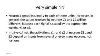
- 15. Very simple NN • Now suppose further that neuron Y is connected to neurons Z1 and Z2 , with weights v1 and v2, respectively. 8/30/2020
- 16. Very simple NN • Neuron Y sends its signal y to each of these units. However, in general, the values received by neurons Z1 and Z2 will be different, because each signal is scaled by the appropriate weight, v1 or v2. • In a typical net, the activations z1 , and z2 of neurons Z1 , and Z2 depend on inputs from several or even many neurons, not just one. 8/30/2020
- 17. Neural networks viewed as directed graph 8/30/2020
- 18. Neural networks viewed as directed graph 8/30/2020
- 19. Biological NN • There is a close analogy between the structure of a biological neuron (i.e., a brain or nerve cell) and the processing element (or artificial neuron) presented in the rest of this book. • A biological neuron has three types of components that are of particular interest in understanding an artificial neuron: its dendrites, soma. and axon. 8/30/2020
- 21. Biological NN • The many dendrites receive signals from other neurons. • The signals are electric impulses that are transmitted across a synaptic gap by means of a chemical process. • The action of the chemical transmitter modifies the incoming signal (typically, by scaling the frequency of the signals that are received) in a manner similar to the action of the weights in an artificial neural network. 8/30/2020
- 22. Biological NN • The soma, or cell body sums the incoming signals. When sufficient input is received, the cell fires; that is, it transmits a signal over its axon to other cells. • It is often supposed that a cell either fires or doesn't at any instant of time, so that transmitted signals can be treated as binary. 8/30/2020
- 23. Biological NN • Several key features of the processing elements of artificial neural networks are suggested by the properties of biological neurons: – 1) The processing element receives many signals. – 2) Signals may be modified by a weight at the receiving synapse. – 3) The processing element sums the weighted inputs. – 4) Under appropriate circumstances (sufficient input), the neuron transmits a single output. 8/30/2020
- 24. Biological NN – 5) The output from a particular neuron may go to many other neurons (the axon branches). – 6) Information processing is local. – 7) Memory is distributed: • a. Long-term memory resides in the neurons' synapses or weights. • b. Short-term memory corresponds to the signals sent by the neurons. 8/30/2020
- 25. Biological NN – 8) A synapse's strength may be modified by experience. – 9) Neurotransmitters for synapses may be excitatory or inhibitory. 8/30/2020
- 26. Biological NN • Biological neural systems are fault tolerant in two respects: a) we are able to recognize many input signals that are somewhat different from any signal we have seen before. –An example of this is our ability to recognize a person in a picture we have not seen before or to recognize a person after a long period of time. b) we are able to tolerate damage to the neural system itself. Humans are born with as many as 100 billion neurons. Most of these are in the brain, and most are not replaced when they die. –In spite of our continuous loss of neurons, we continue to learn. 8/30/2020
- 27. NN Applications • Signal Processing – Noise cancelation in telephone system. • Control – truck backer-upper • Pattern recognition – Handwritten characters • Medicine – Instance physician • Speech production and recognition – NETtalk 8/30/2020
- 28. Typical Architectures • The arrangement of neurons into layers and the connection patterns within and between layers is called the net architecture. • Typically, neurons in the same layer behave in the same manner. • To be more specific, in many neural networks, the neurons within a layer are either fully interconnected or not interconnected at all. • Neural nets are often classified as single layer or multilayer. 8/30/2020
- 30. NN Layers • Input Layer: As the name suggests, it accepts inputs in several different formats provided by the programmer. • Hidden Layer: The hidden layer presents in-between input and output layers. It performs all the calculations to find hidden features and patterns. • Output Layer: The input goes through a series of transformations using the hidden layer, which finally results in output that is conveyed using this layer. 8/30/2020
- 31. Benefits of Artificial Neural Networks • ANNs offers many key benefits that make them particularly well-suited to specific issues and situations: 1. ANNs can learn and model non-linear and complicated interactions, which is critical since many of the relationships between inputs and outputs in real life are non-linear and complex. 2. ANNs can generalize – After learning from the original inputs and their associations, the model may infer unknown relationships from anonymous data, allowing it to generalize and predict unknown data. 3. ANN does not impose any constraints on the input variables, unlike many other prediction approaches (like how they should be distributed). Furthermore, numerous studies have demonstrated that ANNs can better simulate heteroskedasticity, or data with high volatility and non-constant variance, because of their capacity to discover latent correlations in the data without imposing any preset associations. This is particularly helpful in financial time series forecasting (for example, stock prices) when significant data volatility. 8/30/2020
- 32. Advantages of Artificial Neural Network (ANN) • Parallel processing capability: Artificial neural networks have a numerical value that can perform more than one task simultaneously. • Storing data on the entire network: Data that is used in traditional programming is stored on the whole network, not on a database. The disappearance of a couple of pieces of data in one place doesn't prevent the network from working. • Capability to work with incomplete knowledge: After ANN training, the information may produce output even with inadequate data. The loss of performance here relies upon the significance of missing data. • Having a memory distribution: For ANN is to be able to adapt, it is important to determine the examples and to encourage the network according to the desired output by demonstrating these examples to the network. The succession of the network is directly proportional to the chosen instances, and if the event can't appear to the network in all its aspects, it can produce false output. • Having fault tolerance: Extortion of one or more cells of ANN does not prohibit it from generating output, and this feature makes the network fault-tolerance. 8/30/2020
- 33. Disadvantages of Artificial Neural Network • Assurance of proper network structure: There is no particular guideline for determining the structure of artificial neural networks. The appropriate network structure is accomplished through experience, trial, and error. • Unrecognized behavior of the network: It is the most significant issue of ANN. When ANN produces a testing solution, it does not provide insight concerning why and how. It decreases trust in the network. • Hardware dependence: Artificial neural networks need processors with parallel processing power, as per their structure. Therefore, the realization of the equipment is dependent. • Difficulty of showing the issue to the network: ANNs can work with numerical data. Problems must be converted into numerical values before being introduced to ANN. The presentation mechanism to be resolved here will directly impact the performance of the network. It relies on the user's abilities. • The duration of the network is unknown: The network is reduced to a specific value of the error, and this value does not give us optimum results. 8/30/2020
- 34. Types of Artificial Neural Network • Feedback ANN: In this type of ANN, the output returns into the network to accomplish the best-evolved results internally. As per the University of Massachusetts, Lowell Centre for Atmospheric Research. The feedback networks feed information back into itself and are well suited to solve optimization issues. The Internal system error corrections utilize feedback ANNs. • Feed-Forward ANN: A feed-forward network is a basic neural network comprising of an input layer, an output layer, and at least one layer of a neuron. Through assessment of its output by reviewing its input, the intensity of the network can be noticed based on group behavior of the associated neurons, and the output is decided. The primary advantage of this network is that it figures out how to evaluate and recognize input patterns. 8/30/2020
- 38. History of ANN The history of ANN can be divided into the following three eras − ANN during 1940s to 1960s Some key developments of this era are as follows − •1943 It has been assumed that the concept of neural network started with the work of − physiologist, Warren McCulloch, and mathematician, Walter Pitts, when in 1943 they modeled a simple neural network using electrical circuits in order to describe how neurons in the brain might work. •1949 Donald Hebb’s book, − The Organization of Behavior, put forth the fact that repeated activation of one neuron by another increases its strength each time they are used. •1956 An associative memory network was introduced by Taylor. − •1958 A learning method for McCulloch and Pitts neuron model named Perceptron was − invented by Rosenblatt. •1960 Bernard Widrow and Marcian Hoff developed models called "ADALINE" and − “MADALINE.” 8/30/2020
- 39. History of ANN ANN during 1960s to 1980s Some key developments of this era are as follows − •1961 Rosenblatt made an unsuccessful attempt but proposed the − “backpropagation” scheme for multilayer networks. •1964 Taylor constructed a winner-take-all circuit with inhibitions among − output units. •1969 Multilayer perceptron (MLP) was invented by Minsky and Papert. − •1971 Kohonen developed Associative memories. − •1976 Stephen Grossberg and Gail Carpenter developed Adaptive − resonance theory. 8/30/2020
- 40. History of ANN ANN from 1980s till Present Some key developments of this era are as follows − •1982 The major development was Hopfield’s Energy approach. − •1985 Boltzmann machine was developed by Ackley, Hinton, and Sejnowski. − •1986 Rumelhart, Hinton, and Williams introduced Generalised Delta Rule. − •1988 Kosko developed Binary Associative Memory (BAM) and also gave the concept of − Fuzzy Logic in ANN. •The historical review shows that significant progress has been made in this field. Neural network based chips are emerging and applications to complex problems are being developed. Surely, today is a period of transition for neural network technology. 8/30/2020
- 41. Single layer Net • A single-layer net has one layer of connection weights. • the units can be distinguished as input units, which receive signals from the outside world, and output units, from which the response of the net can be read. • For pattern classification, each output unit corresponds to a particular category to which an input vector may or may not belong. • For pattern association. the same architecture can be used, but now the overall pattern of output signals gives the response pattern associated with the input signal that caused it to be produced. 8/30/2020
- 43. Multi-layer Net • the same type of net can be used for different problems, depending on the interpretation of the response of the net. • On the other hand, more complicated mapping problems may require a multilayer network. • A multilayer net is a net with one or more layers (or levels) of nodes (the so called hidden units) between the input units and the output units. • Multilayer nets can solve more complicated problems than can single-layer nets, but training may be more difficult. 8/30/2020
- 45. Competitive layer • A competitive layer forms a part of a large number of neural networks. • Typically, the interconnections between neurons in the competitive layer are not shown in the architecture diagrams for such nets. • The winner-take-all competition, and MAXNET are based on competition. 8/30/2020
- 47. Setting the Weights • in addition to the architecture, the method of setting the values of the weights (training) is an important distinguishing characteristic of different neural nets • For a neural network three types of training is used – Supervised – unsupervised – Fixed 8/30/2020
- 48. Supervised training • In perhaps the most typical neural net setting, training is accomplished by presenting a sequence of training vectors, or patterns, each with an associated target output vector. • The weights are then adjusted according to a learning algorithm. • This process is known as supervised training. • the output is a bivalent element, say, either 1 (if the input vector belongs to the category) or –1 (if it does not belong). 8/30/2020
- 49. Supervised training • Pattern association is another special form of a mapping problem, one in which the desired output is not just a "yes" or "no," but rather a pattern. • A neural net that is trained to associate a set of input vectors with a corresponding set of output vectors is called an associative memory. • If the desired output vector is the same as the input vector, the net is an autoassociative memory; if the output target vector is different from the input vector, the net is a heteroassociative memory. 8/30/2020
- 50. Unsupervised training • Self-organizing neural nets group similar input vectors together without the use of training data to specify what a typical member of each group looks like or to which group each vector belongs. • A sequence of input vectors is provided, but no target vectors are specified. • The neural net will produce an exemplar (representative) vector for each cluster formed. 8/30/2020
- 51. Fixed-weight nets • Still other types of neural nets can solve constrained optimization problems. • Such nets may work well for problems that can cause difficulty for traditional techniques, such as problems with conflicting constraints (i.e., not all constraints can be satisfied simultaneously). • The Boltzmann machine (without learning) and the continuous Hopfield net can be used for constrained optimization problems. 8/30/2020
- 52. Activation Functions • the basic operation of an artificial neuron involves summing its weighted input signal and applying an activation function. • Typically, the same activation function is used for all neurons in any particular layer of a neural net, although, this is not required. • In most cases, a nonlinear activation function is used. 8/30/2020
- 53. Activation Functions • Binary step function. • Binary sigmoid. • Bipolar sigmoid. 8/30/2020
- 54. Binary step function • Single-layer nets often use a step function to convert the net input, which is a continuously valued variable, to an output unit that is a binary (1 or 0) or bipolar (1 or - 1) signal. 8/30/2020
- 55. Binary sigmoid • Sigmoid functions (S-shaped curves) are useful activation functions. • The logistic function and the hyperbolic tangent functions are the most common. • They are especially advantageous for use in neural nets trained by backpropagation, because the simple relationship between the value of the function at a point and the value of the derivative at that point reduces the computational burden during training. 8/30/2020
- 57. Bipolar sigmoid • The logistic sigmoid function can be scaled to have any range of values that is appropriate for a given problem. • The most common range is from - 1 to 1; we call this sigmoid the bipolar sigmoid. 8/30/2020
- 64. McCULLOCH- PITTS • It is one of the first of neural nets. • McCulloch-Pitts neurons may be summarized as: – The activation of a McCulloch-Pitts neuron is binary. That is, at any time step, the neuron either fires (has an activation of 1) or does not fire (has an activation of 0). – neurons are connected by directed, weighted paths. – A connection path is excitatory if the weight on the path is positive; otherwise it is inhibitory. All excitatory connections into a particular neuron have the same weights. 8/30/2020
- 65. McCULLOCH- PITTS – All excitatory connections into a particular neuron have the same weights. – Each neuron has a fixed threshold such that if the net input to the neuron is greater than the threshold, the neuron fires. – The threshold is set so that inhibition is absolute. That is, any nonzero inhibitory input will prevent the neuron from firing. – It takes one time step for a signal to pass over one connection link. 8/30/2020
- 66. McCULLOCH- PITTS The threshold for unit Y is 4 8/30/2020
- 67. McCULLOCH- PITTS In general form: 8/30/2020
- 68. McCULLOCH- PITTS • The condition that inhibition is absolute requires that for the activation function satisfy the inequality: • Y will fire if it receives k or more excitatory inputs and no inhibitory inputs, where: 8/30/2020
- 69. Applications • The condition that inhibition is absolute requires that for the activation function satisfy the inequality: • The weights for a McCulIoch-Pitts neuron are set, together with the threshold for the neuron's activation function, so that the neuron will perform a simple logic function. • Using these simple neurons as building blocks, we can model any function or phenomenon that can be represented as a logic function. 8/30/2020
- 70. AND 8/30/2020
- 71. OR 8/30/2020
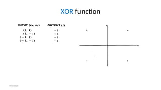
- 73. XOR 8/30/2020
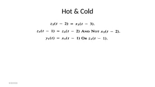
- 74. Hot & Cold • if a cold stimulus is applied to a person's skin for a very short period of time, the person will perceive heat. • However, if the same stimulus is applied for a longer period, the person will perceive cold. • In the figure, neurons XI and X2 represent receptors for heat and cold, respectively, and neurons Y1 and Y2 are the counterpart preceptors. • Neurons Z1and Z2 are auxiliary units needed for the problem • Each neuron has a threshold of 2. 8/30/2020
- 75. Hot & Cold • The desired response of the system is that cold is perceived if a cold stimulus is applied for two time steps, i.e., • heat be perceived if either a hot stimulus is applied or a cold stimulus is applied briefly (for one time step) and then removed. 8/30/2020
- 78. Cold Stimulus (one step) 8/30/2020
- 79. t=1 8/30/2020
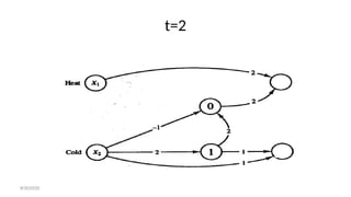
- 80. t=2 8/30/2020
- 81. t=3 8/30/2020
- 82. Cold Stimulus (two step) 8/30/2020
- 83. t=1 8/30/2020
- 84. t=2 8/30/2020
- 85. Hot Stimulus (one step) 8/30/2020
- 86. t=1 8/30/2020
- 88. Inhibitory & Exitatory Action Potential 8/30/2020
- 89. Simple Neural Nets For Pattern Classification 8/30/2020
- 90. General Discussion • One of the simplest tasks that neural nets can be trained to perform is pattern classification. • In pattern classification problems, each input vector (pattern) belongs, or does not belong, to a particular class or category. • For a neural net approach, we assume we have a set of training patterns for which the correct classification is known. • The output unit represents membership in the class with a response of 1; a response of - 1 (or 0 if binary representation is used) indicates that the pattern is not a member of the class. 8/30/2020
- 91. General Discussion • In 1963, neural networks was used to detect heart abnormalities with EKG types of data as input (46 measurements) and classified them into "normal" or "abnormal”. • When patterns may or may not belong to several classes, there is an output unit for each class. • In this chapter, we shall discuss three methods of training a simple single layer neural net for pattern classification: the Hebb rule, the perceptron learning rule, and the delta rule. 8/30/2020
- 92. Architecture • The basic architecture of the simplest possible neural networks that perform pattern classification consists of a layer of input units (as many units as the patterns to be classified have components) and a single output unit. 8/30/2020
- 94. 8/30/2020
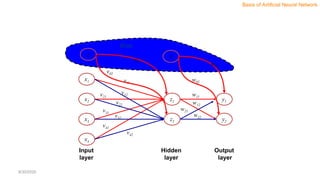
- 95. Architecture • Input layer – It contains those units (Artificial Neurons) which receive input from the outside world on which the network will learn, recognize about or otherwise process. • Output layer – It contains units that respond to the information about how it’s learned any task. • Hidden layer – These units are in between input and output layers. The job of the hidden layer is to transform the input into something that the output unit can use in some way. • Most Neural Networks are fully connected which means to say each hidden neuron is fully linked to every neuron in its previous layer(input) and to the next layer (output) layer. 8/30/2020
- 96. 8/30/2020
- 97. 8/30/2020
- 98. 8/30/2020
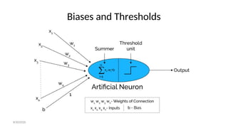
- 99. Biases and Thresholds • A bias acts exactly as a weight on a connection from a unit whose activation is always 1. • Increasing the bias increases the net input to the unit. • If a bias is included, the activation function is typically taken to be: 8/30/2020
- 100. 8/30/2020
- 101. 8/30/2020
- 103. Biases and Thresholds • Some authors do not use a bias weight, but instead use a fixed threshold 0 for the activation function. In that case : 8/30/2020
- 104. The role of a bias and threshold • we consider the separation of the input space into regions where the response of the net is positive and regions where the response is negative. 8/30/2020
- 105. The role of a bias and threshold • The boundary between the values of x1 and x2: • With bias: • With threshold: 8/30/2020
- 106. The role of a bias and threshold • During training, values of w, and w2 are determined so that the net will have the correct response for the training data. • including neither a bias nor a threshold is equivalent to requiring the separating line (or plane or hyperplane for inputs with more components) to pass through the origin. 8/30/2020
- 107. Think… Can you identify which is “the Simpsons”. Learning and Weights..? 8/30/2020
- 108. Learning and Weights..? Learning and Weights..? 8/30/2020
- 109. “the Simpsons” “the not” Learning and Weights..? Learning and Weights..? 8/30/2020
- 110. Learning and Weights..? Learning and Weights..? ID Age Gender Sugar Hypertension Heart Attack 453 78 man 9 mg yes no 226 12 man 13 mg no no 194 15 woman 16 mg no yes 112 17 woman 13 mg yes yes 122 22 woman 7 mg yes yes 789 66 man 8 mg no no Data / Observation / Experience (past experience) ID Age Gender Sugar Hypertension Heart Attack 001 49 man 5 mg yes ???? new data… 8/30/2020
- 111. Hidden layer Output layer Input layer AGE GENDER SUGAR HYPERTENSION HEART ATTACK NO HEART ATTACK Learning and Weights..? Learning and Weights..? w1 w2 wk v1 v2 vj 8/30/2020
- 112. x2 w1 w2 x1 Dendrite Axon yin = x1w1 + x2w2 Nukleus Activation Function: (y-in) = 1 if y-in >= and (y-in) = 0 y - A neuron receives input, determines the strength or the weight of the input, calculates the total weighted input, and compares the total weighted with a value (threshold) -The value is in the range of 0 and 1 - If the total weighted input greater than or equal the threshold value, the neuron will produce the output, and if the total weighted input less than the threshold value, no output will be produced Synapse Learning and Weights..? Learning and Weights..? 8/30/2020
- 113. Input layer Hidden layer Output layer x4 x1 x2 x3 z1 z2 v11 v12 v21 v22 v31 v32 v42 v41 y1 y2 w11 w12 w21 w22 1 1 v01 w01 Bias v02 w02 Basis of Artificial Neural Network 8/30/2020
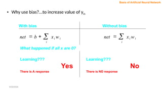
- 114. i i i w x net With bias Without bias i i i w x b net What happened if all x are 0? Learning??? Yes There is A response Learning??? No There is NO response Basis of Artificial Neural Network • Why use bias?...to increase value of yin 8/30/2020
- 115. Weight Initialization and Update Basis of Artificial Neural Network • You may set the initial weights with any values. • The choice of initial weights will influence whether the net reaches a global (or only a local) minimum of the error and how quickly it converges. • Important to avoid choices of initial weights that would make it likely that either activations or its derivatives are zero. • Must not be too large – the initial input signals to each hidden or output unit will be likely to fall in the region where the derivative of the sigmoid func. has a very small value – saturation region. 8/30/2020
- 116. Generating Random Weight Nguyen-Widrow Weights Weights • Must not be too small – The net input to a hidden or output unit will be close to zero – cause extremely slow learning. • Methods Basis of Artificial Neural Network 8/30/2020
- 117. • Random Initialization – A common procedure is to initialize the weights (and biases) to random values between any suitable interval. • Such as –0.5 and 0.5 or –1 and 1. – The values may be +ve or –ve because the final weights after training may be of either sign also. Basis of Artificial Neural Network 8/30/2020
- 118. n number of input units p number of hidden units scale factor: n n p p 7 . 0 ) ( 7 . 0 1 For each hidden unit (j = 1, …, p): Initialize its weight vector (from the input units): vij(old) = random num. between –0.5 and 0.5 Compute || vj(old) || 2 2 2 2 1 ) ( ... ) ( ) ( old v old v old v nj j j n i ij old v 1 2 ) ( 2 1 1 2 ) ( n i ij old v • Nguyen-Widrow Initialization Basis of Artificial Neural Network 8/30/2020
- 119. Reinitialize weights: Set bias: ) ( v ) ( old old v v j ij ij and between num random 0 j v Basis of Artificial Neural Network 8/30/2020
- 120. + positive region - negative region Linear Separability Basis of Artificial Neural Network • The problem is “linear separable” – If there are weights (and a bias) so that all of the training input vectors for which the correct response is +1 lie on one side of the decision boundary and all of the training input vectors for which the correct response is –1 lie on the other side of the decision boundary. 8/30/2020
- 121. • Problem: AND, OR, XOR AND OR XOR 1 0 0 0 0 0 0 1 1 1 1 1 Basis of Artificial Neural Network 8/30/2020
- 122. NEURAL NETWORK WITH SUPERVISED LEARNING (Single Layer Net) 8/30/2020
- 123. Modelling a Simple Problem • Should I attend this lecture? – x1 = weather ( hot or raining) – x2 = day (weekday or weekend) 1 x1 y x2 ? ? ? 8/30/2020
- 124. Example: 2 input AND (bipolar) s0 s1 s2 t 1 1 1 1 1 1 -1 -1 1 -1 1 -1 1 -1 -1 -1 s0 s1 s2 t 1 1 1 1 1 1 0 0 1 0 1 0 1 0 0 0 bipolar binary 8/30/2020
- 125. Hebb’s Rule • Unsupervised learning by Donald Hebb • If 2 neurons on either side of a synapse are activated simultaneously, then the strength of that synapse is selected increased • If 2 neurons on either side of a synapse are activated asynchronously, then the strength of that synapse is selected increased • Time Dependent, Local, Strongly interactive and Correlational • Correlation – a mutual relationship or connection • wi(new) = wi(old) + xi*y 8/30/2020
- 126. Hebb’s Rule • Positive ,negative and uncorrelated state Classification of synaptic modifications 1.Hebbian 2.Ani Hebbian 3.Non -Hebbian 8/30/2020
- 127. Hebb’s Algorithm 1. Set initial weights: wi = 0 for 0 <= i <= n 2. for each training vector 3. set xi = si for all input units 4. set y = t 5. wi(new) = wi(old) + xi*y 8/30/2020
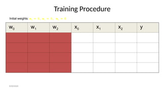
- 128. Training Procedure w0 w1 w2 x0 x1 x2 y Initial weights: w0 = 0, w1 = 0, w2 = 0 8/30/2020
- 129. Result Interpretation • -2 + 2x1 + 2x2 = 0 OR • x2 = -x1 + 1 • This training procedure is order dependent and not guaranteed. 8/30/2020
- 130. Perceptrons (1958) • Very important early neural network • Guaranteed training procedure under certain circumstances 1 x1 y xn w0 w1 wn 8/30/2020
- 131. Activation Function • (yin) = 1 if yin > (yin) = 0 if - <= yin <= (yin) = -1 otherwise 8/30/2020
- 132. Learning Rule • wi(new) = wi(old) + *t*xi if error • is the learning rate • Typically, 0 < <= 1 8/30/2020
- 133. Perceptron’s Algorithm 1. Set initial weights: wi = 0 for 0 <= i <= n (can be random) 2. for each training exemplar do 3. xi = si 4. yin = xi*wi 5. y = f(yin) 6. wi(new) = wi(old) + *t*xi if error 7. if stopping condition not reached, go to 2 f(yin) = 1 if yin > f(yin) = 0 if - <= yin <= f(yin) = -1 otherwise 8/30/2020
- 134. Example: AND concept • bipolar inputs • bipolar target • = 0 • = 1 8/30/2020
- 135. Training Procedure - Epoch 1 w0 w1 w2 x0 x1 x2 yin y t Initial weights: w0 = 0, w1 = 0, w2 = 0 8/30/2020
- 136. Exercise • Continue the above example until the learning is finished. 8/30/2020
- 137. Training Procedure - Epoch 2 w0 w1 w2 x0 x1 x2 yin y t 8/30/2020
- 138. Perceptron Learning Rule Convergence Theorem • If a weight vector exists that correctly classifies all of the training examples, then the perceptron learning rule will converge to some weight vector that gives the correct response for all training patterns. This will happen in a finite number of steps. 8/30/2020
- 139. Comparison between Hebb and Perceptron Hebb Perceptron learning is not iterative Iterative learning Activation Function: -Binary step function without threshold 1 if yin ≥ -1 if yin < 0 Activation Function: - Binari step function with threshold 1 if yin > 0 if - <= yin <= -1 if yin < - Adjustment of weights: wi(new) = wi(old) + xi*y Adjustment of weights: wi(new) = wi(old) + *t*xi Single layer net Single layer net Supervised learning Supervised learning y = f(yin) y = f(yin) 8/30/2020
- 140. Exercise Prepare a Perceptron learning table for epoch 1 and epoch 2 for problem of AND logic with bias using following learning requirements: - bipolar input and target - learning rate, () = 1 - threshold, () = 0.2. 8/30/2020
- 141. Single Layer Net Single Layer Net (Problem Analysis) (Problem Analysis) 8/30/2020
- 143. Problem Description : To predict whether an application of a student to stay in college is accepted, KIV or rejected Problem: Classification 8/30/2020
- 144. Original Data Matric Name Gender CGPA Result 22619 David Male ≥ 3.00 Accepted 22467 John Male 3.00 Rejected 23542 Cathy Female ≥ 3.00 Accepted 24561 Sarah Female 3.00 KIV 8/30/2020
- 145. Original Data (After selected) Gender CGPA Result Male ≥ 3.00 Accepted Male 3.00 Rejected Female ≥ 3.00 Accepted Female 3.00 KIV 8/30/2020
- 146. Representation of Data Gender CGPA Result 1 1 1 1 -1 -1 -1 1 1 -1 -1 0 Gender Male ( 1 ) Female ( -1 ) CGPA ≥ 3.00 ( 1 ) 3.00 ( -1 ) Result Accepted ( 1 ) Rejected ( -1 ) KIV ( 0 ) Data for learning 8/30/2020
- 147. Learning Gender CGPA Result 1 1 1 1 -1 -1 -1 1 1 -1 -1 0 x1 = Gender x2 = CGPA Target = Result Step 1: …… Step 2: …. w0 : ? w1 : ? w2 : ? LEARNING weights Perceptron, Hebb and etc 8/30/2020
- 148. Prediction Gender CGPA 1 1 yin = b + xi*wi 1 if yin > 0 if - <= yin <= -1 if yin < - Matric Name Gender CGPA 43425 Farid Male ≥ 3.00 ( 1 ) Accepted ( -1 ) Rejected ( 0 ) KIV New Data y = PREDICTION x1 = 1 x2 = 1 weights: w0 : ? w1 : ? w2 : ? Binary step function, Binary sigmoid function and etc - depends on problem 8/30/2020
- 149. Linear Separability • For a particular output unit, the desired response is a "yes" if the input pattern is a member of its class and a "no" if it is not. • A "yes" response is represented by an output signal of 1, a "no" by an output signal of - 1 (for bipolar signals). • Since the net input to the output unit is: • the boundary between the region is: 8/30/2020
- 150. Linear Separability • If there are weights (and a bias) so that all of the training input vectors for which the correct response is +1 lie on one side of the decision boundary and all of the training input vectors for which the correct response is -1 lie on the other side of the decision boundary, we say that the problem is "linearly separable." 8/30/2020
- 151. Linear Separability • Minsky and Papert [I988] showed that a single-layer net can learn only linearly separable problems. • Furthermore, it is easy to extend this result to show that multilayer nets with linear activation functions are no more powerful than single-layer nets (since the composition of linear functions is linear). 8/30/2020
- 154. Linear Separability • OR function is also similar to AND function. • The equations of the decision boundaries are not unique. • Note that if a bias weight were not included in these examples, the decision boundary would be forced to go through the origin. • Not all simple two-input, single-output mappings can be solved by a single layer net (even with a bias included), as is illustrated in Example 2.4. 8/30/2020
- 156. Data Representation • Binary or Bipolar • Binary representation is also not as good as bipolar if we want the net to generalize (i.e., respond to input data similar, but not identical to, training data). • Using bipolar input, missing data can be distinguished from mistaken data. Missing values can be represented by "0" and mistakes by reversing the input value from + 1 to - 1, or vice versa. • In general, bipolar representation is preferable 8/30/2020
- 157. HEBB NET • The earliest and simplest learning rule for a neural net is generally known as the Hebb rule. • Hebb proposed that learning occurs by modification of the synapse strengths (weights) in a manner such that if two interconnected neurons are both "on" at the same time, then the weight between those neurons should be increased. • If data are represented in bipolar form, it is easy to express the desired weight update as: 8/30/2020
- 158. HEBB NET • If the data are binary, this formula does not distinguish between a training pair in which an input unit is "on" and the target value is "off" and a training pair in which both the input unit and the target value are "off." 8/30/2020
- 159. Algorithm 8/30/2020
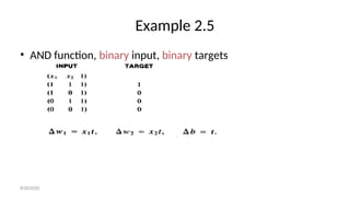
- 160. Example 2.5 • AND function, binary input, binary targets 8/30/2020
- 163. Example 2.7 • AND function, bipolar input, bipolar targets 8/30/2020
- 164. Example 2.7 • First input: 8/30/2020
- 165. Example 2.7 • First input: 8/30/2020
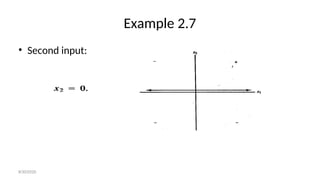
- 166. Example 2.7 • Second input: 8/30/2020
- 167. Example 2.7 • Second input: 8/30/2020
- 168. Example 2.7 • Third input: 8/30/2020
- 169. Example 2.7 • Third input: 8/30/2020
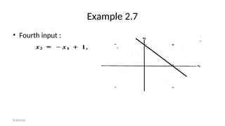
- 170. Example 2.7 • Fourth input: 8/30/2020
- 171. Example 2.7 • Fourth input : 8/30/2020
- 172. Example 2.8 • Character recognition 8/30/2020
- 173. Example 2.8 • The correct response for the first pattern is "on," or + 1, so the weights after presenting the first pattern are simply the input pattern. • The bias weight after presenting this is + 1. • The correct response for the second pattern is "off," or - 1, so the weight change when the second pattern is presented is • 1 -1 -1 -1 1, -1 1 1 1 -1, -1 1 1 1 -1, -1 1 1 1 -1, 1 -1 -1 -1 1. 8/30/2020
- 174. Example 2.8 • In addition, the weight change for the bias weight is - 1. • Adding the weight change to the weights representing the first pattern gives • the final weights: 2 -2 -2 -2 2, -2 2 0 2 -2, -2 2 0 2 -2, -2 2 0 2 -2, -2 2 0 2 -2, 2 -2 -2 -2 2 • The bias weight is 0 8/30/2020
- 175. Example 2.8 • The net input (for any input pattern) is the dot product of the input pattern with the weight vector. • For the first training vector, the net input is 42, so the response is positive, as desired. • For the second training pattern, the net input is -42, so the response is clearly negative, also as desired. 8/30/2020
- 176. Example 2.8 • The first type of change is usually referred to as "mistakes in the data.“ changing a 1 to a - 1, or vice versa. • The second type of change is called "missing data.“ the value 0, rather than 1 or - 1. • In general, a net can handle more missing components than wrong components; in other words, with input data, "It's better not to guess." 8/30/2020
- 177. Example 2.10 • Limitation of Hebb rule training for bipolar patterns. 8/30/2020
- 178. Example 2.10 • Limitation of Hebb rule training for bipolar patterns. 8/30/2020
- 179. Example 2.10 • Again, it is clear that the weights do not give the correct output for the first input pattern. • Figure 2.13 shows that the input points are linearly separable; one possible plane, XI + x2 + x3 + (-2) = 0, to perform the separation is shown. • This plane corresponds to a weight vector of (1 1 1) and a bias of -2. 8/30/2020
- 181. PERCEPTRON • The perceptron learning rule is a more powerful learning rule than the Hebb rule. • Under suitable assumptions, its iterative learning procedure can be proved to converge to the correct weights, i.e., the weights that allow the net to produce the correct output value for each of the training input patterns. 8/30/2020
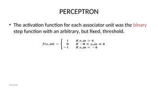
- 182. PERCEPTRON • The activation function for each associator unit was the binary step function with an arbitrary, but fixed, threshold. 8/30/2020
- 183. PERCEPTRON • If an error occurred for a particular training input pattern, the weights would be changed according to the formula • where the target value t is + 1 or - 1 and a is the learning rate. • If an error did not occur, the weights would not be changed. • Training would continue until no error occurred. 8/30/2020
- 185. Algorithm 8/30/2020
- 186. Algorithm 8/30/2020
- 187. Algorithm • Two separating lines: 8/30/2020
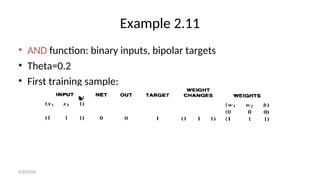
- 188. Example 2.11 • AND function: binary inputs, bipolar targets • Theta=0.2 • First training sample: 8/30/2020
- 190. Example 2.11 • Second training sample: 8/30/2020
- 192. Example 2.11 • Third training sample: • Fourth training sample: 8/30/2020
- 193. Example 2.11 • The response of the all inputs are negative which is not true for the (1,1). So we need more iteration. • After ninth epoch: • After tenth epoch: 8/30/2020
- 194. Example 2.11 • Separating lines are: 8/30/2020
- 195. Example 2.11 • Separating lines are: 8/30/2020
- 196. Example 2.12 • A Perceptron for the AND function: bipolar inputs and targets. • The training process Alpha=1 and threshold and initial weights = 0. 8/30/2020
- 197. Example 2.12 • First epoch: 8/30/2020
- 198. Example 2.12 • Second epoch: • the system was fully trained after the first epoch. • Bipolar representation reduces number of epochs. 8/30/2020
- 200. Training for several output neurons 8/30/2020
- 201. Training for several output neurons 8/30/2020
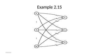
- 202. Example 2.15 • We want to classify the following 21 characters written by 3 fonts into 7 classes. 8/30/2020
- 209. 8/30/2020
- 210. 8/30/2020
- 211. 8/30/2020
- 212. 8/30/2020
- 213. 8/30/2020
- 214. 8/30/2020
- 215. 8/30/2020
- 216. 8/30/2020
- 217. 8/30/2020
- 218. 8/30/2020
- 219. 8/30/2020
- 220. 8/30/2020
- 221. 8/30/2020
- 222. 8/30/2020
- 223. 8/30/2020
- 224. 8/30/2020
- 225. 8/30/2020
- 226. 8/30/2020
- 227. 8/30/2020
- 228. 8/30/2020
- 229. 8/30/2020
- 230. 8/30/2020
- 231. 8/30/2020
- 232. 8/30/2020
- 233. 8/30/2020
- 234. 8/30/2020
- 235. ARTIFICIAL NEURAL NETWORK MATLAB IMPLEMENTATION 8/30/2020
- 236. Steps of Developing ANN Model • Loading the data set • Separating the data set into Training and Testing • Defining the network structure • Setting initial values for weights and bias • Initializing the network • Training the network • Testing the network • Displaying the result 8/30/2020
- 237. Loading the data set • Clear the console – clc • Clear the workspace variables – clear all • Close the child/figure windows – close all • Load the data – load irisdata.m; • Create the data into a matrix – XY=irisdata; 8/30/2020
- 238. Data Separation • Separate the input – X=XY(:,1:4); • Separate the output – Y=XY(:,5:7); • Divide the testing input and output – X2 = X(1:2:150,:); – Y2 = Y(1:2:150,:); • Divide the training input and output – X([1:2:150],:)=[]; – Y([1:2:150],:)=[]; – X1 = X; – Y1 = Y; 8/30/2020
- 239. Data Normalization – Y2n=Y2 8/30/2020 • Min-Max Normalization – minX1=min(X1); – maxX1=max(X1); – for i=1:size(X1,1) • for j=1:size(X1,2) – X1n(i,j)=(X1(i,j)-minX1(j))/(maxX1(j)-minX1(j)); • end – end – Similarly do it for creating x2n from x2 – Y1n=Y1 8/30/2020
- 240. Creating the Network • PR=[min(X); max(X)]'; • nhid=4; • nout=3; • net = newff(PR,[nhid nout],{'tansig‘ 'purelin'},'trainscg','learngdm','mse'); • rand('seed',0); • net.layers{1}.initFcn='initwb'; • net.inputWeights{1,1}.initFcn='rands'; • net.biases{1,1}.initFcn='rands'; • net.biases{2,1}.initFcn='rands'; • net=init(net); 8/30/2020 6
- 241. Training the Network • net.trainParam.epochs =1200; • net.trainParam.goal = 0.01; • [net TR] = train(net,X1n',Y1n'); • MseTr=TR.perf(size(TR.perf,2)) • Time=cputime-t • W1=net.IW{1,1}; • b1=net.b{1,1}; • W2=net.LW{2}; • b2=net.b{2}; 8/30/2020
- 242. Testing the Network • [y]=sim(net,X2n'); • E=Y2n'-y;; • MseTe=mse(E) • n=size(y,1); • m=size(y,2); • for i=1:n – for j=1:m • if y(i,j)>0.5 – y(i,j)=1; • else – y(i,j)=0; • end – end • end 8/30/2020
- 243. Display the Result • y=y'; • n=size(y,1); • for i=1:n • if y(i,:)==[1 0 0]; • s(i)=1; • elseif y(i,:)==[0 1 0]; • s(i)=2; • else y(i,:)==[0 0 1]; • s(i)=3; • end • if Y2(i,:)==[1 0 0]; • a(i)=1; • elseif Y2(i,:)==[0 1 0]; • a(i)=2; • else Y2(i,:)==[0 0 1]; • a(i)=3; • end • end • cc=0; • for i=1:75 • if (s(i)==a(i)) • cc=cc+1; • end • end • cc • plot(s,'bo'); • hold on; • plot(a,'rx'); • title('Actual output = x Network output=o') 8/30/2020 243
- 244. 8/30/2020 244
- 245. Neural Networks Toolbox Analysis and Design
- 246. Matlab Neural Networks Toolbox The neural network toolbox makes it easier to use neural networks in matlab. The toolbox consists of a set of functions and structures that handle neural networks: activation functions training algorithms, etc. The Neural Network Toolbox is contained in a directory called nnet. Type help nnet for a listing of help topics.
- 247. The Structure of the Neural Network Toolbox (I) The toolbox is based on the network object. This object contains information about everything that concern the neural network: the number of its layers the structure of its layers the connectivity between the layers, etc. Matlab provides high-level network creation functions, like: newlin (create a linear layer) newp (create a perceptron) newff (create a feed-forward backpropagation network)
- 248. The Structure of the Neural Network Toolbox (II - Example) NEWFF Create a feed-forward backpropagation network. >>P = [0 1 2 3 4 5 6 7 8 9 10]; (INPUTS) >>T = [0 1 2 3 4 3 2 1 2 3 4]; (TARGETS) Here a two-layer feed-forward network is created. The network's input ranges from [0 to 10]. The first layer has five TANSIG neurons, the second layer has one PURELIN neuron. The TRAINLM network training function is to be used. >>net = newff(minmax(P),[5 1],{'tansig' 'purelin'});
- 249. The Structure of the Neural Network Toolbox (II – Example Cont.) Here the network is simulated and its output plotted against the targets. >>Y = sim(net,P); >>plot(P,T,P,Y,'o') Here the network is trained for 50 epochs. Again the network's output is plotted. >>net.trainParam.epochs = 50; >>net = train(net,P,T); >>Y = sim(net,P); >>plot(P,T,P,Y,'o')
- 250. The Structure of the Neural Network Toolbox (III) Type: >>net First the architecture parameters and the subobject structures subobject structures: inputs: {1x1 cell} of inputs layers: {1x1 cell} of layers outputs: {1x1 cell} containing 1 output targets: {1x1 cell} containing 1 target biases: {1x1 cell} containing 1 bias inputWeights: {1x1 cell} containing 1 input weight layerWeights: {1x1 cell} containing no layer weights are shown. The latter contains information about the individual objects of the network.
- 251. The Structure of the Neural Network Toolbox (IV) The next paragraph contains the training, initialization and performance functions. functions: adaptFcn: ’trains’ initFcn: ’initlay’ performFcn: ’mse’ trainFcn: ’trainc’ The trainFcn and adaptFcn are used for the two different learning types batch learning and incremental or on-line learning. The ANN toolbox include almost 20 training functions.
- 252. The Structure of the Neural Network Toolbox (V) >> net.trainFcn = ’mytrainingfun’; The parameters of the training functions: parameters: adaptParam: .passes initParam: (none) performParam: (none) trainParam: .epochs, .goal, .show, .time The weights and biases are also stored in the network structure: weight and bias values: IW: {1x1 cell} containing 1 input weight matrix LW: {1x1 cell} containing no layer weight matrices b: {1x1 cell} containing 1 bias vector
- 253. Neural Network using NN Toolbox V5.0 To implement a Neural Network, 7 steps must be followed: 1. Loading data source. 2. Selecting attributes required. 3. Decide training, validation, and testing data. 4. Data manipulations and Target generation. (for supervised learning) 5. Neural Network creation (selection of network architecture) and initialisation. 6. Network Training and Testing. 7. Performance evaluation.
- 254. Neural Network Fitting Tool GUI Open the Neural Network Fitting Tool window with this command: >>nftool
- 255. Loading Data Source Load Input Data from workspace Load Target Data from workspace Data description
- 256. Decide training, validation, and testing data. Divide Data Set in subsets for Training and Validation
- 257. Selecting Attributes Select the Number of Neurons
- 259. Training and Performance Evaluation Mean Squared Error
- 260. Saving Results
Editor's Notes
- #1: NOTE: Want a different image on this slide? Select the picture and delete it. Now click the Pictures icon in the placeholder to insert your own image.