Bayesian Nonparametrics: Models Based on the Dirichlet Process
8 likes2,084 views

This document summarizes an introduction to Bayesian nonparametric models presented by Alessandro Panella. It discusses Bayesian learning and De Finetti's theorem, which shows that any exchangeable sequence of random variables can be represented as conditionally independent given a random variable. Finite mixture models are introduced as a Bayesian approach to clustering. Dirichlet process mixture models provide a nonparametric generalization that allows for an unbounded number of clusters.


![Introduction and background Bayesian learning
A simple example
Infer the bias θ ∈ [0, 1] of a coin after observing N tosses.
H = 1, T = 0, p(H) = θ
h = θ, hence H = [0, 1]
Sequence of Bernoulli trials: θ
p(x1 , . . . , xn |θ) = θnH (1 − θ)N−nH x1 x2 xN
where nH = # heads.
Unknown θ: θ
1
p(x1 , . . . , xN ) = θnH (1 − θ)nH −k p(θ) dθ xi
0
N
Need to find a “good” prior p(θ). . .
Beta distribution!
Alessandro Panella (CS Dept. - UIC) Bayesian Nonparametrics February 18, 2013 10 / 57](https://image.slidesharecdn.com/nonparametricbayes-130329120556-phpapp01/85/Bayesian-Nonparametrics-Models-Based-on-the-Dirichlet-Process-16-320.jpg)


![Dirichlet process mixture models The Dirichlet process
The Dirichlet process (cont’d)
D IRICHLET P ROCESS
A draw G ∼ DP(α, H) is an infinite discrete probability measure:
All clusters can contain more than one 5
∞ element ⇒ θ only contains atoms: 4.5
G(θ) = where θ = w δ
4
πk δ(θ, θk ), ∞
j φ∗
j
3.5
3
G
k=1 j=1 2.5
2
What is the prior on {wj , φ∗ }?
θk ∼ H, and π is sampled from a “stick-breaking prior.”
1.5
j
1
Stick-breaking representation: 0.5
0
0 0.1 0.2 0.3 0.4 0.5 0.6 0.7 0.8 0.9 1
j−1
φ∗ ∼ H
j
Θ (from Orbanz Teh, 2008)
wj = vj (1 − vj )
vj ∼ Beta(1, α) i=1
w1
Break a stick Masses decreasing on average: GEM
distribution.
w4
w3
w2
Imagine a stick of length one. For k = 1 . . . ∞, do the following:
Strictly decreasing masses: Poisson-Dirichlet
distribution.
Break the stick at a point drawn from Beta(1, α).
[Kin75, Set94]
Let πk be such value and keep the remainder of the stick.
Peter Orbanz Yee Whye Teh 50 / 71
Following standard convention, we write π ∼ GEM(α).
(Details in second part of talk)
Alessandro Panella (CS Dept. - UIC) Bayesian Nonparametrics February 18, 2013 29 / 57](https://image.slidesharecdn.com/nonparametricbayes-130329120556-phpapp01/85/Bayesian-Nonparametrics-Models-Based-on-the-Dirichlet-Process-44-320.jpg)
![Dirichlet process mixture models The Dirichlet process
The Dirichlet process (cont’d)
D IRICHLET P ROCESS
A draw G ∼ DP(α, H) is an infinite discrete probability measure:
All clusters can contain more than one 5
∞ element ⇒ θ only contains atoms: 4.5
G(θ) = where θ = w δ
4
πk δ(θ, θk ), ∞
j φ∗
j
3.5
3
G
k=1 j=1 2.5
2
What is the prior on {wj , φ∗ }?
θk ∼ H, and π is sampled from a “stick-breaking prior.”
1.5
j
1
Stick-breaking representation: 0.5
0
0 0.1 0.2 0.3 0.4 0.5 0.6 0.7 0.8 0.9 1
j−1
φ∗ ∼ H
j
Θ (from Orbanz Teh, 2008)
wj = vj (1 − vj )
vj ∼ Beta(1, α) i=1
w1
Break a stick Masses decreasing on average: GEM
distribution.
w4
w3
w2
Imagine a stick of length one. For k = 1 . . . ∞, do the following:
Strictly decreasing masses: Poisson-Dirichlet
distribution.
Break the stick at a point drawn from Beta(1, α).
[Kin75, Set94]
Let πk be such value and keep the remainder of the stick.
Peter Orbanz Yee Whye Teh 50 / 71
Following standard convention, we write π ∼ GEM(α).
(Details in second part of talk)
Alessandro Panella (CS Dept. - UIC) Bayesian Nonparametrics February 18, 2013 29 / 57](https://image.slidesharecdn.com/nonparametricbayes-130329120556-phpapp01/85/Bayesian-Nonparametrics-Models-Based-on-the-Dirichlet-Process-45-320.jpg)
![Dirichlet process mixture models The Dirichlet process
Stick-breaking, intuitively
Sec. 2.5. Dirichlet Processes 101
0.5 0.5
β1 1−β1 0.4 0.4
π1 0.3 0.3
k
k
β2 1−β2
!
!
0.2 0.2
π2 β3 1−β3
0.1
0
0 5 10 15 20
0.1
0
0 5 10 15 20
k k
π3 β4 1−β4
0.5
0.4
0.5
0.4
π4 0.3 0.3
k
k
!
!
β5 0.2 0.2
π5 0.1
0
0 5 10 15 20
0.1
0
0 5 10 15 20
k k
α=1 α=5
(from Sudderth, 2008)
Figure 2.22. Sequential stick–breaking construction of the infinite set of mixture weights π ∼ GEM(α)
corresponding to a measure G ∼ DP(α, H). Left: The first weight π1 ∼ Beta(1, α). Each subsequent
weight πk (red) is some random proportion βk (blue) of the remaining, unbroken “stick” of probability
Small α ⇒ lots first weight assigned to few random stick–breaking constructions (two
mass. Right: The of K = 20 weights generated by four θk ’s.
⇒ G will be very different from base measure H.
with α = 1, two with α = 5). Note that the weights πk do not monotonically decrease.
Large α ⇒ weights equally distributed on θk ’s. N , there are strong bounds
discrete parameters {θk }∞ . For a given α and dataset size
k=1
on the accuracy of resemble the truncations of this stick–breaking process [147],
⇒ G will particular finite base measure H.
which are often used in approximate computational methods [29, 147, 148, 289].
Several other stick–breaking processes have been proposed which sample the pro-
portions βk from different distributions [147, 148, 233]. For example, the two–parameter
Alessandro Panella (CS Dept. - UIC) Bayesian Nonparametrics February 18, 2013 30 / 57](https://image.slidesharecdn.com/nonparametricbayes-130329120556-phpapp01/85/Bayesian-Nonparametrics-Models-Based-on-the-Dirichlet-Process-46-320.jpg)


![A little more theory. . . Dirichlet process REDUX
Dirichlet Process REDUX
Definition
Let Θ be a measurable space (of parameters), H be a probability distribution
on Θ, and α a positive scalar. A Dirichlet process is the distribution of a
random probability measure G over Θ, such that for any finite partition
(T1 , . . . , Tk ) of Θ, we have
(G(T1 ), . . . , G(TK )) ∼ Dir(αH(T1 ), . . . , αH(TK )).
Sec. 2.5. Dirichlet Processes 97
~
T2
Θ T1 ~ ~
T1 T3
T3 ~
T2 T4
~
T5
(from Sudderth, 2008)
Figure 2.21. Dirichlet processes induce Dirichlet distributions on every finite, measurable partition.
Left: An example base measure H on a bounded, two–dimensional space Θ (darker regions have higher
E[G(T )] = H(T )
probability). Center: A partition with K = 3 cells. The weight that a random measure G ∼ DP(α, H)
k k
assigns to these cells follows a Dirichlet distribution (see eq. (2.166)). We shade each cell Tk according
to its mean E[G(Tk )] = H(Tk ). Right: Another partition with K = 5 cells. The consistency of G
Alessandro Panella (CS Dept. - UIC) Bayesian Nonparametrics
e February 18, 2013 41 / 57](https://image.slidesharecdn.com/nonparametricbayes-130329120556-phpapp01/85/Bayesian-Nonparametrics-Models-Based-on-the-Dirichlet-Process-62-320.jpg)


![A little more theory. . . Dirichlet process REDUX
Stick-breaking (derivation) [Teh 2007]
We know that (posterior):
G ∼ DP(α, H) θ ∼H
⇔
θ|G ∼ G G|θ ∼ DP α + 1, αH+δθ
α+1
Consider the partition (Θ, Θ θ) of Θ. We have:
αH + δθ αH + δθ
(G(Θ), G(Θ θ)) ∼ Dir (α + 1) (θ), (α + 1) (Θ θ)
α+1 α+1
= Dir(1, α) = Beta(1, α)
G has point mass located at θ:
G = βδθ + (1 − β)G β ∼ Beta(1, α)
and G is the renormalized probability measure with the point mass
removedÉ
What is G ?
Alessandro Panella (CS Dept. - UIC) Bayesian Nonparametrics February 18, 2013 44 / 57](https://image.slidesharecdn.com/nonparametricbayes-130329120556-phpapp01/85/Bayesian-Nonparametrics-Models-Based-on-the-Dirichlet-Process-65-320.jpg)
![A little more theory. . . Dirichlet process REDUX
Stick-breaking (derivation) [Teh 2007]
We know that (posterior):
G ∼ DP(α, H) θ ∼H
⇔
θ|G ∼ G G|θ ∼ DP α + 1, αH+δθ
α+1
Consider the partition (Θ, Θ θ) of Θ. We have:
αH + δθ αH + δθ
(G(Θ), G(Θ θ)) ∼ Dir (α + 1) (θ), (α + 1) (Θ θ)
α+1 α+1
= Dir(1, α) = Beta(1, α)
G has point mass located at θ:
G = βδθ + (1 − β)G β ∼ Beta(1, α)
and G is the renormalized probability measure with the point mass
removedÉ
What is G ?
Alessandro Panella (CS Dept. - UIC) Bayesian Nonparametrics February 18, 2013 44 / 57](https://image.slidesharecdn.com/nonparametricbayes-130329120556-phpapp01/85/Bayesian-Nonparametrics-Models-Based-on-the-Dirichlet-Process-66-320.jpg)
![A little more theory. . . Dirichlet process REDUX
Stick-breaking (derivation) [Teh 2007]
We know that (posterior):
G ∼ DP(α, H) θ ∼H
⇔
θ|G ∼ G G|θ ∼ DP α + 1, αH+δθ
α+1
Consider the partition (Θ, Θ θ) of Θ. We have:
αH + δθ αH + δθ
(G(Θ), G(Θ θ)) ∼ Dir (α + 1) (θ), (α + 1) (Θ θ)
α+1 α+1
= Dir(1, α) = Beta(1, α)
G has point mass located at θ:
G = βδθ + (1 − β)G β ∼ Beta(1, α)
and G is the renormalized probability measure with the point mass
removedÉ
What is G ?
Alessandro Panella (CS Dept. - UIC) Bayesian Nonparametrics February 18, 2013 44 / 57](https://image.slidesharecdn.com/nonparametricbayes-130329120556-phpapp01/85/Bayesian-Nonparametrics-Models-Based-on-the-Dirichlet-Process-67-320.jpg)
![A little more theory. . . Dirichlet process REDUX
Stick-breaking (derivation) [Teh 2007]
We know that (posterior):
G ∼ DP(α, H) θ ∼H
⇔
θ|G ∼ G G|θ ∼ DP α + 1, αH+δθ
α+1
Consider the partition (Θ, Θ θ) of Θ. We have:
αH + δθ αH + δθ
(G(Θ), G(Θ θ)) ∼ Dir (α + 1) (θ), (α + 1) (Θ θ)
α+1 α+1
= Dir(1, α) = Beta(1, α)
G has point mass located at θ:
G = βδθ + (1 − β)G β ∼ Beta(1, α)
and G is the renormalized probability measure with the point mass
removedÉ
What is G ?
Alessandro Panella (CS Dept. - UIC) Bayesian Nonparametrics February 18, 2013 44 / 57](https://image.slidesharecdn.com/nonparametricbayes-130329120556-phpapp01/85/Bayesian-Nonparametrics-Models-Based-on-the-Dirichlet-Process-68-320.jpg)
![A little more theory. . . Dirichlet process REDUX
Stick-breaking (derivation) [Teh 2007]
We have:
θ ∼H
G ∼ DP(α, H) G|θ ∼ DP α + 1, αH+δθ
α+1
⇒
θ|G ∼G G = βδθ + (1 − β)G
β ∼ Beta(1, α)
Consider a further partition θ, T1 , . . . , TK ) of Θ:
(G(θ), G(T1 ), . . . , G(TK )) = (β, (1 − β)G (T1 ), . . . , (1 − β)G (TK ))
∼ Dir(1, αH(T1 ), . . . , αH(TK ))
Using the agglomerative/decimative property of Dirichlet, we get
(G (T1 ), . . . , G (TK )) ∼ Dir(αH(T1 ), . . . , αH(TK ))
G ∼ DP(α, H)
Alessandro Panella (CS Dept. - UIC) Bayesian Nonparametrics February 18, 2013 45 / 57](https://image.slidesharecdn.com/nonparametricbayes-130329120556-phpapp01/85/Bayesian-Nonparametrics-Models-Based-on-the-Dirichlet-Process-69-320.jpg)
![A little more theory. . . Dirichlet process REDUX
Stick-breaking (derivation) [Teh 2007]
We have:
θ ∼H
G ∼ DP(α, H) G|θ ∼ DP α + 1, αH+δθ
α+1
⇒
θ|G ∼G G = βδθ + (1 − β)G
β ∼ Beta(1, α)
Consider a further partition θ, T1 , . . . , TK ) of Θ:
(G(θ), G(T1 ), . . . , G(TK )) = (β, (1 − β)G (T1 ), . . . , (1 − β)G (TK ))
∼ Dir(1, αH(T1 ), . . . , αH(TK ))
Using the agglomerative/decimative property of Dirichlet, we get
(G (T1 ), . . . , G (TK )) ∼ Dir(αH(T1 ), . . . , αH(TK ))
G ∼ DP(α, H)
Alessandro Panella (CS Dept. - UIC) Bayesian Nonparametrics February 18, 2013 45 / 57](https://image.slidesharecdn.com/nonparametricbayes-130329120556-phpapp01/85/Bayesian-Nonparametrics-Models-Based-on-the-Dirichlet-Process-70-320.jpg)
![A little more theory. . . Dirichlet process REDUX
Stick-breaking (derivation) [Teh 2007]
We have:
θ ∼H
G ∼ DP(α, H) G|θ ∼ DP α + 1, αH+δθ
α+1
⇒
θ|G ∼G G = βδθ + (1 − β)G
β ∼ Beta(1, α)
Consider a further partition θ, T1 , . . . , TK ) of Θ:
(G(θ), G(T1 ), . . . , G(TK )) = (β, (1 − β)G (T1 ), . . . , (1 − β)G (TK ))
∼ Dir(1, αH(T1 ), . . . , αH(TK ))
Using the agglomerative/decimative property of Dirichlet, we get
(G (T1 ), . . . , G (TK )) ∼ Dir(αH(T1 ), . . . , αH(TK ))
G ∼ DP(α, H)
Alessandro Panella (CS Dept. - UIC) Bayesian Nonparametrics February 18, 2013 45 / 57](https://image.slidesharecdn.com/nonparametricbayes-130329120556-phpapp01/85/Bayesian-Nonparametrics-Models-Based-on-the-Dirichlet-Process-71-320.jpg)
![A little more theory. . . Dirichlet process REDUX
Stick-breaking (derivation) [Teh 2007]
Therefore,
G ∼ DP(α, H)
G = β1 δθ1 + (1 − β1 )G1
G = β1 δθ1 + (1 − β1 )(β2 δθ2 + (1 − β2 )G2 )
.
.
.
∞
G= πk δθk
k=1
where
k−1
π k = βk (1 − βl ) βl ∼ Beta(1, α),
l=1
which is the stick-breaking construction.
Alessandro Panella (CS Dept. - UIC) Bayesian Nonparametrics February 18, 2013 46 / 57](https://image.slidesharecdn.com/nonparametricbayes-130329120556-phpapp01/85/Bayesian-Nonparametrics-Models-Based-on-the-Dirichlet-Process-72-320.jpg)


![A little more theory. . . Dirichlet process REDUX
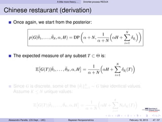
Chinese restaurant (derivation)
A bit informally. . .
Let Tk contain θk and shrink it arbitrarily. To the limit, we have that
K
¯ ¯ ¯ 1
p(θN+1 = θ|θ1 , . . . , θN , α, H) = αh(θ) + Nk δθi (θ)
¯
α+N
i=1
This is the generalized Polya urn scheme
An urn contains one ball for each preceding observation, with a different color
for each distinct θk . For each ball drawn from the urn, we replace that ball and
add one more ball of the same color. There is a special “weighted” ball which
is drawn with probability proportional to α normal balls, and has a new,
previously unseen color θ¯. [This description is from Sudderth, 2008]
k
This allows to sample from a Dirichlet process without explicitly
constructing the underlying G ∼ DP(α, H).
Alessandro Panella (CS Dept. - UIC) Bayesian Nonparametrics February 18, 2013 48 / 57](https://image.slidesharecdn.com/nonparametricbayes-130329120556-phpapp01/85/Bayesian-Nonparametrics-Models-Based-on-the-Dirichlet-Process-76-320.jpg)
![A little more theory. . . Dirichlet process REDUX
Chinese restaurant (derivation)
A bit informally. . .
Let Tk contain θk and shrink it arbitrarily. To the limit, we have that
K
¯ ¯ ¯ 1
p(θN+1 = θ|θ1 , . . . , θN , α, H) = αh(θ) + Nk δθi (θ)
¯
α+N
i=1
This is the generalized Polya urn scheme
An urn contains one ball for each preceding observation, with a different color
for each distinct θk . For each ball drawn from the urn, we replace that ball and
add one more ball of the same color. There is a special “weighted” ball which
is drawn with probability proportional to α normal balls, and has a new,
previously unseen color θ¯. [This description is from Sudderth, 2008]
k
This allows to sample from a Dirichlet process without explicitly
constructing the underlying G ∼ DP(α, H).
Alessandro Panella (CS Dept. - UIC) Bayesian Nonparametrics February 18, 2013 48 / 57](https://image.slidesharecdn.com/nonparametricbayes-130329120556-phpapp01/85/Bayesian-Nonparametrics-Models-Based-on-the-Dirichlet-Process-77-320.jpg)


Bayesian Nonparametrics: Models Based on the Dirichlet Process
- 1. Bayesian Nonparametrics: Models Based on the Dirichlet Process Alessandro Panella Department of Computer Science University of Illinois at Chicago Machine Learning Seminar Series February 18, 2013 Alessandro Panella (CS Dept. - UIC) Bayesian Nonparametrics February 18, 2013 1 / 57
- 2. Sources and Inspirations Tutorials (slides) P. Orbanz and Y.W. Teh, Modern Bayesian Nonparametrics. NIPS 2011. M. Jordan, Dirichlet Process, Chinese Restaurant Process, and All That. NIPS 2005. Articles etc. E.B. Sudderth, Chapter in PhD thesis, 2006. E. Fox, Chapter in PhD thesis, 2008. Y.W. Teh, Dirichlet Processes. Encyclopedia of Machine Learning, 2010. Springer. ... Alessandro Panella (CS Dept. - UIC) Bayesian Nonparametrics February 18, 2013 2 / 57
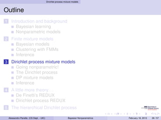
- 3. Outline 1 Introduction and background Bayesian learning Nonparametric models 2 Finite mixture models Bayesian models Clustering with FMMs Inference 3 Dirichlet process mixture models Going nonparametric! The Dirichlet process DP mixture models Inference 4 A little more theory. . . De Finetti’s REDUX Dirichlet process REDUX 5 The hierarchical Dirichlet process Alessandro Panella (CS Dept. - UIC) Bayesian Nonparametrics February 18, 2013 3 / 57
- 4. Introduction and background Outline 1 Introduction and background Bayesian learning Nonparametric models 2 Finite mixture models Bayesian models Clustering with FMMs Inference 3 Dirichlet process mixture models Going nonparametric! The Dirichlet process DP mixture models Inference 4 A little more theory. . . De Finetti’s REDUX Dirichlet process REDUX 5 The hierarchical Dirichlet process Alessandro Panella (CS Dept. - UIC) Bayesian Nonparametrics February 18, 2013 4 / 57
- 5. Introduction and background Bayesian learning The meaning of it all BAYESIAN NONPARAMETRICS Alessandro Panella (CS Dept. - UIC) Bayesian Nonparametrics February 18, 2013 5 / 57
- 6. Introduction and background Bayesian learning The meaning of it all BAYESIAN NONPARAMETRICS Alessandro Panella (CS Dept. - UIC) Bayesian Nonparametrics February 18, 2013 5 / 57
- 7. Introduction and background Bayesian learning The meaning of it all BAYESIAN NONPARAMETRICS Alessandro Panella (CS Dept. - UIC) Bayesian Nonparametrics February 18, 2013 5 / 57
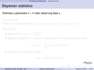
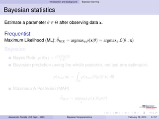
- 8. Introduction and background Bayesian learning Bayesian statistics Estimate a parameter θ ∈ Θ after observing data x. Frequentist ˆ Maximum Likelihood (ML): θMLE = argmaxθ p(x|θ) = argmaxθ L(θ : x) Bayesian p(x|θ)p(θ) Bayes Rule: p(θ|x) = p(x) Bayesian prediction (using the whole posterior, not just one estimator) p(xnew |x) = p(xnew |θ)p(θ|x) dθ Θ Maximum A Posteriori (MAP) ˆ θMAP = argmax p(x|θ)p(θ) θ Alessandro Panella (CS Dept. - UIC) Bayesian Nonparametrics February 18, 2013 6 / 57
- 9. Introduction and background Bayesian learning Bayesian statistics Estimate a parameter θ ∈ Θ after observing data x. Frequentist ˆ Maximum Likelihood (ML): θMLE = argmaxθ p(x|θ) = argmaxθ L(θ : x) Bayesian p(x|θ)p(θ) Bayes Rule: p(θ|x) = p(x) Bayesian prediction (using the whole posterior, not just one estimator) p(xnew |x) = p(xnew |θ)p(θ|x) dθ Θ Maximum A Posteriori (MAP) ˆ θMAP = argmax p(x|θ)p(θ) θ Alessandro Panella (CS Dept. - UIC) Bayesian Nonparametrics February 18, 2013 6 / 57
- 10. Introduction and background Bayesian learning Bayesian statistics Estimate a parameter θ ∈ Θ after observing data x. Frequentist ˆ Maximum Likelihood (ML): θMLE = argmaxθ p(x|θ) = argmaxθ L(θ : x) Bayesian p(x|θ)p(θ) Bayes Rule: p(θ|x) = p(x) Bayesian prediction (using the whole posterior, not just one estimator) p(xnew |x) = p(xnew |θ)p(θ|x) dθ Θ Maximum A Posteriori (MAP) ˆ θMAP = argmax p(x|θ)p(θ) θ Alessandro Panella (CS Dept. - UIC) Bayesian Nonparametrics February 18, 2013 6 / 57
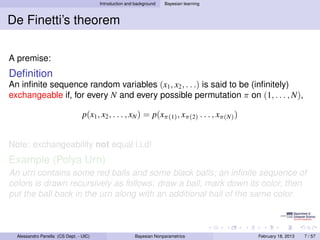
- 11. Introduction and background Bayesian learning De Finetti’s theorem A premise: Definition An infinite sequence random variables (x1 , x2 , . . .) is said to be (infinitely) exchangeable if, for every N and every possible permutation π on (1, . . . , N), p(x1 , x2 , . . . , xN ) = p(xπ(1) , xπ(2) . . . , xπ(N) ) Note: exchangeability not equal i.i.d! Example (Polya Urn) An urn contains some red balls and some black balls; an infinite sequence of colors is drawn recursively as follows: draw a ball, mark down its color, then put the ball back in the urn along with an additional ball of the same color. Alessandro Panella (CS Dept. - UIC) Bayesian Nonparametrics February 18, 2013 7 / 57
- 12. Introduction and background Bayesian learning De Finetti’s theorem A premise: Definition An infinite sequence random variables (x1 , x2 , . . .) is said to be (infinitely) exchangeable if, for every N and every possible permutation π on (1, . . . , N), p(x1 , x2 , . . . , xN ) = p(xπ(1) , xπ(2) . . . , xπ(N) ) Note: exchangeability not equal i.i.d! Example (Polya Urn) An urn contains some red balls and some black balls; an infinite sequence of colors is drawn recursively as follows: draw a ball, mark down its color, then put the ball back in the urn along with an additional ball of the same color. Alessandro Panella (CS Dept. - UIC) Bayesian Nonparametrics February 18, 2013 7 / 57
- 13. Introduction and background Bayesian learning De Finetti’s theorem (cont’d) Theorem (De Finetti, 1935. Aka Representation Theorem) A sequence of random variables (x1 , x2 , . . .) is infinitely exchangeable if for all N, there exists a random variable θ and a probability measure p on it such that N p(x1 , x2 , . . . , xN ) = p(θ) p(xi |θ) dθ Θ i=1 i.e., there exists a parameter space and a measure on it that makes the variables iid! The representation theorem motivates (and encourages!) the use of Bayesian statistics. Alessandro Panella (CS Dept. - UIC) Bayesian Nonparametrics February 18, 2013 8 / 57
- 14. Introduction and background Bayesian learning De Finetti’s theorem (cont’d) Theorem (De Finetti, 1935. Aka Representation Theorem) A sequence of random variables (x1 , x2 , . . .) is infinitely exchangeable if for all N, there exists a random variable θ and a probability measure p on it such that N p(x1 , x2 , . . . , xN ) = p(θ) p(xi |θ) dθ Θ i=1 i.e., there exists a parameter space and a measure on it that makes the variables iid! The representation theorem motivates (and encourages!) the use of Bayesian statistics. Alessandro Panella (CS Dept. - UIC) Bayesian Nonparametrics February 18, 2013 8 / 57
- 15. Introduction and background Bayesian learning Bayesian learning Hypothesis space H Given data D, compute p(D|h)p(h) p(h|D) = p(D) Then, we probably want to predict some future data D , by either: Average over H, i.e. p(D |D) = H p(D |h)p(h|D)p(h) dh Choose the MAP h (or compute it directly), i.e. p(D |D) = p(D |hMAP ) Sample from the posterior ... H can be anything! Bayesian learning as a general learning framework We will consider the case in which h is a probabilistic model itself, i.e. a parameter vector θ. Alessandro Panella (CS Dept. - UIC) Bayesian Nonparametrics February 18, 2013 9 / 57
- 16. Introduction and background Bayesian learning A simple example Infer the bias θ ∈ [0, 1] of a coin after observing N tosses. H = 1, T = 0, p(H) = θ h = θ, hence H = [0, 1] Sequence of Bernoulli trials: θ p(x1 , . . . , xn |θ) = θnH (1 − θ)N−nH x1 x2 xN where nH = # heads. Unknown θ: θ 1 p(x1 , . . . , xN ) = θnH (1 − θ)nH −k p(θ) dθ xi 0 N Need to find a “good” prior p(θ). . . Beta distribution! Alessandro Panella (CS Dept. - UIC) Bayesian Nonparametrics February 18, 2013 10 / 57
- 17. Introduction and background Bayesian learning A simple example (cont’d) Beta distribution: θ ∼ Beta(a, b) 1 a−1 p(θ|a, b) = B(a,b) θ (1 − θ)b−1 Bayesian learning: p(h|D) ∝ p(D|h)p(h); for us: Beta(0.1, 0.1) p(θ|x1 , . . . , xN ) ∝ p(x1 , . . . , xn |θ)p(θ) 1 = θnH (1 − θ)nT θa−1 (1 − θ)b−1 Beta(1, 1) B(a, b) ∝ θnH +a−1 (1 − θ)nT +b−1 i.e. θ|x1 , . . . , xN ∼ Beta(a + NH , b + NT ) Beta(2, 3) We’re lucky! The Beta distribution is a conjugate prior to the binomial distribution. Beta(10, 10) Alessandro Panella (CS Dept. - UIC) Bayesian Nonparametrics February 18, 2013 11 / 57
- 18. Introduction and background Bayesian learning A simple example (cont’d) Beta distribution: θ ∼ Beta(a, b) 1 a−1 p(θ|a, b) = B(a,b) θ (1 − θ)b−1 Bayesian learning: p(h|D) ∝ p(D|h)p(h); for us: Beta(0.1, 0.1) p(θ|x1 , . . . , xN ) ∝ p(x1 , . . . , xn |θ)p(θ) 1 = θnH (1 − θ)nT θa−1 (1 − θ)b−1 Beta(1, 1) B(a, b) ∝ θnH +a−1 (1 − θ)nT +b−1 i.e. θ|x1 , . . . , xN ∼ Beta(a + NH , b + NT ) Beta(2, 3) We’re lucky! The Beta distribution is a conjugate prior to the binomial distribution. Beta(10, 10) Alessandro Panella (CS Dept. - UIC) Bayesian Nonparametrics February 18, 2013 11 / 57
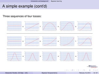
- 19. Introduction and background Bayesian learning A simple example (cont’d) Three sequences of four tosses: H T H H H H H T H H H H Alessandro Panella (CS Dept. - UIC) Bayesian Nonparametrics February 18, 2013 12 / 57
- 20. 8 Introduction and background CHAPTER Nonparametric models 4. NONPARAMETRIC TECHNIQUES Nonparametric models h = .5 h = .2 h=1 “Nonparametric” doesn’t mean “no parameters”! Rather, 4 0.6 The number of parameters grows as more data are observed. 0.15 3 T ERMINOLOGY 0.1 0.4 δ(x) 2 ∞-dimensional parameter space. δ(x) δ(x) 1 2 0.05 0.2 2 2 1 Finite Parametric model number of parameters 1 1 0 data ⇒ Bounded 0 0 -2 0 -2 0 -2 0 -1 -1 -1 0 -1 -1 -1 0 0 Number of parameters fixed (or constantly bounded) w.r.t. sample size 1 1 1 2 -2 2 -2 2 -2 Definition Nonparametric model4.3: Examples of two-dimensional circularly symmetric normal Parzen windows Figure A nonparametric model is a Bayesiandifferent values of anNote that because the δk (·) are normalized, ϕ(x/h) for three model on h. ∞-dimensional parameter Number of parameters grows withscales must be used to show their structure. different vertical sample size space. ∞-dimensional parameter space Example Example: Density estimation 20 CHAPTER 2. BAYESIAN DECISION THEORY x2 p(x) p(x) p(x) µ x1 Parametric Figure 4.4: Three Parzen-windowNonparametric Figure 2.9: Samples drawn from a two-dimensional Gaussian lie in a cloud centered on the mean µ. The red ellipses show lines of equal probability density of the Gaussian. density estimates based on the same set of five Peter Orbanz Yee Whye Teh (from Orbanz and window functions in Fig. 4.3. As before, the71vertical axes have 4/ 2 samples, using the Teh, NIPS 2011) being merely σ times the identity matrix I. Geometrically, this corresponds to the situation in which the samples fall in equal-size hyperspherical to show the structure of each function. been scaled clusters, the cluster for the ith class being centered about the mean vector µ . The computation of the i determinant and the inverse of Σi is particularly easy: |Σi | = σ 2d and Σ−1 = (1/σ 2 )I. i Since both |Σi | and the (d/2) ln 2π term in Eq. 47 are independent of i, they are Alessandro Panella (CS Dept.additive constants unimportant - UIC) Bayesian Nonparametrics that can be ignored. Thus we obtain the simple February 18, 2013 13 / 57
- 21. 8 Introduction and background CHAPTER Nonparametric models 4. NONPARAMETRIC TECHNIQUES Nonparametric models h = .5 h = .2 h=1 “Nonparametric” doesn’t mean “no parameters”! Rather, 4 0.6 The number of parameters grows as more data are observed. 0.15 3 T ERMINOLOGY 0.1 0.4 δ(x) 2 ∞-dimensional parameter space. δ(x) δ(x) 1 2 0.05 0.2 2 2 1 Finite Parametric model number of parameters 1 1 0 data ⇒ Bounded 0 0 -2 0 -2 0 -2 0 -1 -1 -1 0 -1 -1 -1 0 0 Number of parameters fixed (or constantly bounded) w.r.t. sample size 1 1 1 2 -2 2 -2 2 -2 Definition Nonparametric model4.3: Examples of two-dimensional circularly symmetric normal Parzen windows Figure A nonparametric model is a Bayesiandifferent values of anNote that because the δk (·) are normalized, ϕ(x/h) for three model on h. ∞-dimensional parameter Number of parameters grows withscales must be used to show their structure. different vertical sample size space. ∞-dimensional parameter space Example Example: Density estimation 20 CHAPTER 2. BAYESIAN DECISION THEORY x2 p(x) p(x) p(x) µ x1 Parametric Figure 4.4: Three Parzen-windowNonparametric Figure 2.9: Samples drawn from a two-dimensional Gaussian lie in a cloud centered on the mean µ. The red ellipses show lines of equal probability density of the Gaussian. density estimates based on the same set of five Peter Orbanz Yee Whye Teh (from Orbanz and window functions in Fig. 4.3. As before, the71vertical axes have 4/ 2 samples, using the Teh, NIPS 2011) being merely σ times the identity matrix I. Geometrically, this corresponds to the situation in which the samples fall in equal-size hyperspherical to show the structure of each function. been scaled clusters, the cluster for the ith class being centered about the mean vector µ . The computation of the i determinant and the inverse of Σi is particularly easy: |Σi | = σ 2d and Σ−1 = (1/σ 2 )I. i Since both |Σi | and the (d/2) ln 2π term in Eq. 47 are independent of i, they are Alessandro Panella (CS Dept.additive constants unimportant - UIC) Bayesian Nonparametrics that can be ignored. Thus we obtain the simple February 18, 2013 13 / 57
- 22. Finite mixture models Outline 1 Introduction and background Bayesian learning Nonparametric models 2 Finite mixture models Bayesian models Clustering with FMMs Inference 3 Dirichlet process mixture models Going nonparametric! The Dirichlet process DP mixture models Inference 4 A little more theory. . . De Finetti’s REDUX Dirichlet process REDUX 5 The hierarchical Dirichlet process Alessandro Panella (CS Dept. - UIC) Bayesian Nonparametrics February 18, 2013 14 / 57
- 23. Finite mixture models Bayesian models Models in Bayesian data analysis Model Generative process. Expresses how we think the data is generated. Contains hidden variables (the subject of p(θ) learning.) θ M Specifies relations between variables. E.g. graphical models. p(D|M, θ) Posterior inference Knowing p(D|M, θ). . . ← “how data is generated” D . . . compute p(θ|M, D) Akin to “reversing” the generative process. Alessandro Panella (CS Dept. - UIC) Bayesian Nonparametrics February 18, 2013 15 / 57
- 24. Finite mixture models Bayesian models Models in Bayesian data analysis Model Generative process. Expresses how we think the data is generated. Contains hidden variables (the subject of p(θ) learning.) θ M Specifies relations between variables. E.g. graphical models. p(D|M, θ) p(θ|D, M ) Posterior inference Knowing p(D|M, θ). . . ← “how data is generated” D . . . compute p(θ|M, D) Akin to “reversing” the generative process. Alessandro Panella (CS Dept. - UIC) Bayesian Nonparametrics February 18, 2013 15 / 57
- 25. Finite mixture models Clustering with FMMs Finite mixture models (FMMs) Bayesian approach to clustering. Each data point is assumed to belong to one of K clusters. General form A sequence of data points x = (x1 , . . . , xN ) each with probability K p(xi |π, θ1 , . . . , θK ) = πk f (xi |θk ) π ∈ ΠK−1 k=1 Generative process For each i: Draw a cluster assignment zi ∼ π Draw a data point xi ∼ F(θzi ). Alessandro Panella (CS Dept. - UIC) Bayesian Nonparametrics February 18, 2013 16 / 57
- 26. Finite mixture models Clustering with FMMs FMMs (example) Mixture of univariate Gaussians K θk = (µk , σk ) p(xi |π, µ, σ) = πk fN (xi ; µk , σk ) xi ∼ N (µk , σk ) k=1 0.35 0.3 π = (0.15, 0.25, 0.6) 0.25 0.2 0.15 0.1 N (1, 1) N (4, .5) N (6, .7) 0.05 0 −2 0 2 4 6 8 10 Alessandro Panella (CS Dept. - UIC) Bayesian Nonparametrics February 18, 2013 17 / 57
- 27. Finite mixture models Clustering with FMMs FMMs (cont’d) Clustering with FFMs Need priors for π, θ Usually, π is given a (symmetric) Dirichlet distribution prior. θk ’s are given a suitable prior H, depending on the data. α π H π ∼ Dir(α/K, . . . , α/K) zi θk |H ∼ H k = 1...K θk zi |π ∼ π K xi |θ, zi ∼ F(θzi ) i = 1...N xi N Alessandro Panella (CS Dept. - UIC) Bayesian Nonparametrics February 18, 2013 18 / 57
- 28. Finite mixture models Clustering with FMMs Dirichlet distribution Multivariate generalization of Beta. Dirichlet Distributions Dir(1, 1, 1) Dir(2, 2, 2) Dir(5, 5, 5) Dir(5, 5, 2) Dir(5, 2, 2) Dir(0.7, 0.7, 0.7) (from Teh, MLSC 2008) Alessandro Panella (CS Dept. - UIC) Bayesian Nonparametrics February 18, 2013 19 / 57
- 29. Finite mixture models Clustering with FMMs Dirichlet distribution (cont’d) K Γ(α) α/K−1 π ∼ Dir(α/K, . . . , α/K) iff p(π1 , . . . , πK ) = πk k Γ(α/K) k=1 Conjugate prior to categorical/multinomial, i.e. π ∼ Dir( α , . . . , α ) K K zi ∼ π i = 1 . . . N implies α α α π|z1 , . . . , zN ∼ Dir + n1 , + n2 , . . . , + nK K K K Moreover, K Γ(α) Γ(nk + α/K) p(z1 , . . . , zN |α) = Γ(α + N) Γ(α/K) k=1 and (−i) nk + α/K p(zi = k|z(−i) , α) = α+N−1 Alessandro Panella (CS Dept. - UIC) Bayesian Nonparametrics February 18, 2013 20 / 57
- 30. Finite mixture models Inference Inference in FMMs Clustering: infer z (marginalize over π, θ) p(x|z, H)p(z|α) p(z|x, α, H) = , where α π H z p(x|z, H)p(z|α) K Γ(α) Γ(nk + α/K) zi p(z|α) = θk Γ(α + N) k=1 Γ(α/K) K N K p(x|z, H) = p(xi |θzi ) H(θk ) dθ xi Θ i=1 k=1 N Parameter estimation: infer π, θ K p(π, θ|x, α, H) = p(π|z, α) p(θk |x, H) p(z|x, α, H) z k=1 ⇒ No analytic procedure. Alessandro Panella (CS Dept. - UIC) Bayesian Nonparametrics February 18, 2013 21 / 57
- 31. Finite mixture models Inference Inference in FMMs Clustering: infer z (marginalize over π, θ) p(x|z, H)p(z|α) p(z|x, α, H) = , where α π H z p(x|z, H)p(z|α) K Γ(α) Γ(nk + α/K) zi p(z|α) = θk Γ(α + N) k=1 Γ(α/K) K N K p(x|z, H) = p(xi |θzi ) H(θk ) dθ xi Θ i=1 k=1 N Parameter estimation: infer π, θ K p(π, θ|x, α, H) = p(π|z, α) p(θk |x, H) p(z|x, α, H) z k=1 ⇒ No analytic procedure. Alessandro Panella (CS Dept. - UIC) Bayesian Nonparametrics February 18, 2013 21 / 57
- 32. Finite mixture models Inference Inference in FMMs Clustering: infer z (marginalize over π, θ) p(x|z, H)p(z|α) p(z|x, α, H) = , where α π H z p(x|z, H)p(z|α) K Γ(α) Γ(nk + α/K) zi p(z|α) = θk Γ(α + N) k=1 Γ(α/K) K N K p(x|z, H) = p(xi |θzi ) H(θk ) dθ xi Θ i=1 k=1 N Parameter estimation: infer π, θ K p(π, θ|x, α, H) = p(π|z, α) p(θk |x, H) p(z|x, α, H) z k=1 ⇒ No analytic procedure. Alessandro Panella (CS Dept. - UIC) Bayesian Nonparametrics February 18, 2013 21 / 57
- 33. Finite mixture models Inference Inference in FMMs Clustering: infer z (marginalize over π, θ) p(x|z, H)p(z|α) p(z|x, α, H) = , where α π H z p(x|z, H)p(z|α) K Γ(α) Γ(nk + α/K) zi p(z|α) = θk Γ(α + N) k=1 Γ(α/K) K N K p(x|z, H) = p(xi |θzi ) H(θk ) dθ xi Θ i=1 k=1 N Parameter estimation: infer π, θ K p(π, θ|x, α, H) = p(π|z, α) p(θk |x, H) p(z|x, α, H) z k=1 ⇒ No analytic procedure. Alessandro Panella (CS Dept. - UIC) Bayesian Nonparametrics February 18, 2013 21 / 57
- 34. Finite mixture models Inference Inference in FMMs Clustering: infer z (marginalize over π, θ) p(x|z, H)p(z|α) p(z|x, α, H) = , where α π H z p(x|z, H)p(z|α) K Γ(α) Γ(nk + α/K) zi p(z|α) = θk Γ(α + N) k=1 Γ(α/K) K N K p(x|z, H) = p(xi |θzi ) H(θk ) dθ xi Θ i=1 k=1 N Parameter estimation: infer π, θ K p(π, θ|x, α, H) = p(π|z, α) p(θk |x, H) p(z|x, α, H) z k=1 ⇒ No analytic procedure. Alessandro Panella (CS Dept. - UIC) Bayesian Nonparametrics February 18, 2013 21 / 57
- 35. Finite mixture models Inference Approximate inference for FMMs No exact inference because of the unknown clusters identifiers z Expectation-Maximization (EM) Widely used, but we will focus on MCMC because of the connection with Dirichlet Process. Gibbs sampling Markov chain Monte Carlo (MCMC) integration method Set of random variables v = {v1 , v2 , . . . , vM }. We want to compute p(v). Randomly initialize their values. At each iteration, sample a variable vi and hold the rest constant: (t) (t−1) vi ∼ p(vi |vj , j = i) ← usually tractable (t) (t−1) vj = vj This creates a Markov chain with p(v) as equilibrium distribution. Alessandro Panella (CS Dept. - UIC) Bayesian Nonparametrics February 18, 2013 22 / 57
- 36. Finite mixture models Inference Gibbs sampling for FMMs State variables: z1 , . . . , zN , θ1 , . . . , θK , π. Conditional distributions: α α p(π|z, θ) = Dir + n1 , . . . , + nk K K p(θk |x, z) ∝ p(θk ) p(xi |θk ) i:zi =k α π H = H(θk ) Fθk (xi ) i:zi =k zi θk p(zi = k|π, θ, x) ∝ p(zi = k|πk )p(xi |zi = k, θk ) K = πk Fθk (xi ) xi We can avoid sampling π: N p(zi = k|z−i , θ, x) ∝ p(xi |θk )p(zi = k|z−i ) (−i) ∝ Fθk (xi ) nk + α/K Alessandro Panella (CS Dept. - UIC) Bayesian Nonparametrics February 18, 2013 23 / 57
- 37. Finite mixture models Inference Gibbs sampling for FMMs (example) log p(x | !, ) = −539.17 l Mixture of 4 bivariate Gaussians Normal-inverse Wishart prior on θk = (µk , Σk ), conjugate to normal distribution. Σk ∼ W(ν, ∆) µk ∼ N (ϑ, Σk /κ) log p(x | !, ) = −539.17 log p(x | |!, ) = −497.77 log p(x !, ) = −404.18 l T=2 T=10 T=40 log p(x | !, ) = −539.17 log p(x | |!, ) = −497.77 log p(x !, ) = −404.18 log p(x | |!, ) = −454.15 log p(x !, (from Sudderth, 2008) ) = −397.40 l Figure 2.18. Learning a mixture of K = 4 Gaussians using the show the current parameters after T=2 (top), T=10 (middle), and random initializations. Each plot is labeled by the current data lo Alessandro Panella (CS Dept. - UIC) Bayesian Nonparametrics February 18, 2013 24 / 57
- 38. Finite mixture models Inference FMMs: alternative representation 58 CHAPTER 2. NONPARAMETRIC AND GRAPHICAL MODELS H H α π H α zi π θk λ αα G G K ¯ θ2 θ1 xi zi θk θ θii K N xi xii x x x 2 1 N NN π ∼ Dir(α) K θk ∼ H Figure 2.9. Directed graphical representations of a K component mixture model. Mixture weights G(θ) = θk ∼ H in which z ∼ π is the cluster that generates k δ(θ, (θ k ) Right: Alternative π θ π ∼ Dir(α), while cluster parameters are assigned independent priors θk ∼ H(λ). Left: Indicator variable representation, i xi ∼ F z ). π ∼ Dir(α) k=1 i ziof form, ¯ distributional∼ π in which G is a discrete distribution on Θ taking K distinct values. θi ∼ G are the ¯ parameters ¯ θi ∼ G the cluster that generates xi ∼ F (θi ). We illustrate with a mixture of K = 4 Gaussians, where cluster∼ F(θ ) known (bottom) and H(λ) is a Gaussian prior on cluster means (top). xi variancesiθare , and corresponding Gaussians, are shown for two observations x , x . z¯ ,θ Sampled cluster means 1 ¯2 ¯ xi ∼ F(θi ) 1 2 The unobserved indicator variable zi ∈ {1, . . . , K} specifies the unique cluster associated Alessandro Panella Mixture UIC) with xi . (CS Dept. - models are widely Bayesianfor unsupervised learning, where clusters are 2013 used Nonparametrics February 18, 25 / 57
- 39. Dirichlet process mixture models Outline 1 Introduction and background Bayesian learning Nonparametric models 2 Finite mixture models Bayesian models Clustering with FMMs Inference 3 Dirichlet process mixture models Going nonparametric! The Dirichlet process DP mixture models Inference 4 A little more theory. . . De Finetti’s REDUX Dirichlet process REDUX 5 The hierarchical Dirichlet process Alessandro Panella (CS Dept. - UIC) Bayesian Nonparametrics February 18, 2013 26 / 57
- 40. Dirichlet process mixture models Going nonparametric! Going nonparametric! The problem with finite FMMs What if K is unknown? How many parameters? Idea Let’s use ∞ parameters! We want something of the kind: ∞ p(xi |π, θ1 , θ2 , . . .) = πk p(xi |θk ) k=1 How to define such a measure? We’d like the nice conjugancy properties of Dirichlet to carry on. . . Is there such a thing, the ∞ limit of a Dirichlet? Alessandro Panella (CS Dept. - UIC) Bayesian Nonparametrics February 18, 2013 27 / 57
- 41. Dirichlet process mixture models Going nonparametric! Going nonparametric! The problem with finite FMMs What if K is unknown? How many parameters? Idea Let’s use ∞ parameters! We want something of the kind: ∞ p(xi |π, θ1 , θ2 , . . .) = πk p(xi |θk ) k=1 How to define such a measure? We’d like the nice conjugancy properties of Dirichlet to carry on. . . Is there such a thing, the ∞ limit of a Dirichlet? Alessandro Panella (CS Dept. - UIC) Bayesian Nonparametrics February 18, 2013 27 / 57
- 42. Dirichlet process mixture models Going nonparametric! Going nonparametric! The problem with finite FMMs What if K is unknown? How many parameters? Idea Let’s use ∞ parameters! We want something of the kind: ∞ p(xi |π, θ1 , θ2 , . . .) = πk p(xi |θk ) k=1 How to define such a measure? We’d like the nice conjugancy properties of Dirichlet to carry on. . . Is there such a thing, the ∞ limit of a Dirichlet? Alessandro Panella (CS Dept. - UIC) Bayesian Nonparametrics February 18, 2013 27 / 57
- 43. Dirichlet process mixture models The Dirichlet process The (practical) Dirichlet process The Dirichlet process is a distribution over probability measures over Θ. DP(α, H) H(θ) is the base (mean) measure. Think µ for a Gaussian. . . . . . but in the space of probability measures. α is the concentration parameter. Controls the dispersion around the mean H. Alessandro Panella (CS Dept. - UIC) Bayesian Nonparametrics February 18, 2013 28 / 57
- 44. Dirichlet process mixture models The Dirichlet process The Dirichlet process (cont’d) D IRICHLET P ROCESS A draw G ∼ DP(α, H) is an infinite discrete probability measure: All clusters can contain more than one 5 ∞ element ⇒ θ only contains atoms: 4.5 G(θ) = where θ = w δ 4 πk δ(θ, θk ), ∞ j φ∗ j 3.5 3 G k=1 j=1 2.5 2 What is the prior on {wj , φ∗ }? θk ∼ H, and π is sampled from a “stick-breaking prior.” 1.5 j 1 Stick-breaking representation: 0.5 0 0 0.1 0.2 0.3 0.4 0.5 0.6 0.7 0.8 0.9 1 j−1 φ∗ ∼ H j Θ (from Orbanz Teh, 2008) wj = vj (1 − vj ) vj ∼ Beta(1, α) i=1 w1 Break a stick Masses decreasing on average: GEM distribution. w4 w3 w2 Imagine a stick of length one. For k = 1 . . . ∞, do the following: Strictly decreasing masses: Poisson-Dirichlet distribution. Break the stick at a point drawn from Beta(1, α). [Kin75, Set94] Let πk be such value and keep the remainder of the stick. Peter Orbanz Yee Whye Teh 50 / 71 Following standard convention, we write π ∼ GEM(α). (Details in second part of talk) Alessandro Panella (CS Dept. - UIC) Bayesian Nonparametrics February 18, 2013 29 / 57
- 45. Dirichlet process mixture models The Dirichlet process The Dirichlet process (cont’d) D IRICHLET P ROCESS A draw G ∼ DP(α, H) is an infinite discrete probability measure: All clusters can contain more than one 5 ∞ element ⇒ θ only contains atoms: 4.5 G(θ) = where θ = w δ 4 πk δ(θ, θk ), ∞ j φ∗ j 3.5 3 G k=1 j=1 2.5 2 What is the prior on {wj , φ∗ }? θk ∼ H, and π is sampled from a “stick-breaking prior.” 1.5 j 1 Stick-breaking representation: 0.5 0 0 0.1 0.2 0.3 0.4 0.5 0.6 0.7 0.8 0.9 1 j−1 φ∗ ∼ H j Θ (from Orbanz Teh, 2008) wj = vj (1 − vj ) vj ∼ Beta(1, α) i=1 w1 Break a stick Masses decreasing on average: GEM distribution. w4 w3 w2 Imagine a stick of length one. For k = 1 . . . ∞, do the following: Strictly decreasing masses: Poisson-Dirichlet distribution. Break the stick at a point drawn from Beta(1, α). [Kin75, Set94] Let πk be such value and keep the remainder of the stick. Peter Orbanz Yee Whye Teh 50 / 71 Following standard convention, we write π ∼ GEM(α). (Details in second part of talk) Alessandro Panella (CS Dept. - UIC) Bayesian Nonparametrics February 18, 2013 29 / 57
- 46. Dirichlet process mixture models The Dirichlet process Stick-breaking, intuitively Sec. 2.5. Dirichlet Processes 101 0.5 0.5 β1 1−β1 0.4 0.4 π1 0.3 0.3 k k β2 1−β2 ! ! 0.2 0.2 π2 β3 1−β3 0.1 0 0 5 10 15 20 0.1 0 0 5 10 15 20 k k π3 β4 1−β4 0.5 0.4 0.5 0.4 π4 0.3 0.3 k k ! ! β5 0.2 0.2 π5 0.1 0 0 5 10 15 20 0.1 0 0 5 10 15 20 k k α=1 α=5 (from Sudderth, 2008) Figure 2.22. Sequential stick–breaking construction of the infinite set of mixture weights π ∼ GEM(α) corresponding to a measure G ∼ DP(α, H). Left: The first weight π1 ∼ Beta(1, α). Each subsequent weight πk (red) is some random proportion βk (blue) of the remaining, unbroken “stick” of probability Small α ⇒ lots first weight assigned to few random stick–breaking constructions (two mass. Right: The of K = 20 weights generated by four θk ’s. ⇒ G will be very different from base measure H. with α = 1, two with α = 5). Note that the weights πk do not monotonically decrease. Large α ⇒ weights equally distributed on θk ’s. N , there are strong bounds discrete parameters {θk }∞ . For a given α and dataset size k=1 on the accuracy of resemble the truncations of this stick–breaking process [147], ⇒ G will particular finite base measure H. which are often used in approximate computational methods [29, 147, 148, 289]. Several other stick–breaking processes have been proposed which sample the pro- portions βk from different distributions [147, 148, 233]. For example, the two–parameter Alessandro Panella (CS Dept. - UIC) Bayesian Nonparametrics February 18, 2013 30 / 57
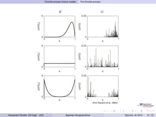
- 47. Dirichlet process mixture models The Dirichlet process H G (from Navarro et al., 2005) Alessandro Panella (CS Dept. - UIC) Bayesian Nonparametrics February 18, 2013 31 / 57
- 48. Dirichlet process mixture models DP mixture models The DP mixture model (DPMM) Let’s use G ∼ DP(α, H) to build an infinite mixture model. 105 HH αα GG G ∼ DP(α, H) ¯ θi ∼ G ¯ θ2 θ1 θθi i xi ∼ Fθi ¯ xxi i x2 x1 N N an infinite, Dirichlet process mixture model. Mix- process, while cluster parameters are assigned in- able representation, in which zi ∼ π is the cluster tributional form, in which G is an infinite discrete ¯ he cluster that generates xi ∼ F (θi ). We illustrate iances are known (bottom) and H(λ) is a Gaussian ¯ ¯Alessandro Panella (CS Dept. - UIC) Bayesian Nonparametrics February 18, 2013 32 / 57
- 49. Dirichlet process mixture models DP mixture models DPM (cont’d) Using explicit clusters indicators z = (z1 , z2 , . . . , zN ). α π H π ∼ GEM(α) θk ∼ H k = 1, . . . , ∞ zi θk ∞ zi ∼ π xi ∼ Fθzi i = 1, . . . , N xi N Alessandro Panella (CS Dept. - UIC) Bayesian Nonparametrics February 18, 2013 33 / 57
- 50. Dirichlet process mixture models DP mixture models Chinese restaurant process So far, we only have a generative model. Is there a “nice” conjugancy property to use during inference? It turns out (details in part 2) that, if π ∼ GEM(α) zi ∼ π the distribution p(z|α) = p(z|π)p(π) dπ is easily tractable, and is known as the Chinese restaurant process (CRP). Alessandro Panella (CS Dept. - UIC) Bayesian Nonparametrics February 18, 2013 34 / 57
- 51. Dirichlet process mixture models DP mixture models Chinese restaurant process (cont’d) Restaurant with ∞ tables with ∞ capacity. 1 2 3 4 ... zi = table at which customer i sits upon entering. Customer 1 sits at table 1 nk p(zi = k) = Customer 2 sits: α+i−1 at table 1 w. prob ∝ 1 α at table 2 w. prob. ∝ α p(zi = knew ) = α+i−1 Customer i sits: at table k w. prob. ∝ nk (# ppl at k) at new table w. prob. ∝ α Alessandro Panella (CS Dept. - UIC) Bayesian Nonparametrics February 18, 2013 35 / 57
- 52. Dirichlet process mixture models DP mixture models Chinese restaurant process (cont’d) Restaurant with ∞ tables with ∞ capacity. 1 1 2 3 4 ... zi = table at which customer i sits upon entering. Customer 1 sits at table 1 nk p(zi = k) = Customer 2 sits: α+i−1 at table 1 w. prob ∝ 1 α at table 2 w. prob. ∝ α p(zi = knew ) = α+i−1 Customer i sits: at table k w. prob. ∝ nk (# ppl at k) at new table w. prob. ∝ α Alessandro Panella (CS Dept. - UIC) Bayesian Nonparametrics February 18, 2013 35 / 57
- 53. Dirichlet process mixture models DP mixture models Chinese restaurant process (cont’d) Restaurant with ∞ tables with ∞ capacity. 1 2 1 2 3 4 ... zi = table at which customer i sits upon entering. Customer 1 sits at table 1 nk p(zi = k) = Customer 2 sits: α+i−1 at table 1 w. prob ∝ 1 α at table 2 w. prob. ∝ α p(zi = knew ) = α+i−1 Customer i sits: at table k w. prob. ∝ nk (# ppl at k) at new table w. prob. ∝ α Alessandro Panella (CS Dept. - UIC) Bayesian Nonparametrics February 18, 2013 35 / 57
- 54. Dirichlet process mixture models DP mixture models Chinese restaurant process (cont’d) Restaurant with ∞ tables with ∞ capacity. 3 1 2 1 2 3 4 ... zi = table at which customer i sits upon entering. Customer 1 sits at table 1 nk p(zi = k) = Customer 2 sits: α+i−1 at table 1 w. prob ∝ 1 α at table 2 w. prob. ∝ α p(zi = knew ) = α+i−1 Customer i sits: at table k w. prob. ∝ nk (# ppl at k) at new table w. prob. ∝ α Alessandro Panella (CS Dept. - UIC) Bayesian Nonparametrics February 18, 2013 35 / 57
- 55. Dirichlet process mixture models DP mixture models Chinese restaurant process (cont’d) Restaurant with ∞ tables with ∞ capacity. 3 5 1 2 7 1 2 3 4 ... 4 6 zi = table at which customer i sits upon entering. Customer 1 sits at table 1 nk p(zi = k) = Customer 2 sits: α+i−1 at table 1 w. prob ∝ 1 α at table 2 w. prob. ∝ α p(zi = knew ) = α+i−1 Customer i sits: at table k w. prob. ∝ nk (# ppl at k) at new table w. prob. ∝ α Alessandro Panella (CS Dept. - UIC) Bayesian Nonparametrics February 18, 2013 35 / 57
- 56. Dirichlet process mixture models Inference Gibbs sampling for DPMMs Via the CRP, we can find the conditional distributions for Gibbs sampling. State: θ1 , . . . , θk , z. p(θk |x, z) ∝ p(θk ) p(xi |θk ) i:zi =k α π H = h(θk )f (xi |θk ) zi θk ∞ p(zi = k|z−i , θ, x) ∝ p(xi |θk )p(zi = k|z−i ) xi (−i) nk f (xi |θk ) exising k N ∝ α f (xi |θk ) new k K grows as more data are observed, asymptotically as α log n. Alessandro Panella (CS Dept. - UIC) Bayesian Nonparametrics February 18, 2013 36 / 57
- 57. Dirichlet process mixture models !, ) Inference log p(x | = −462.25 log p(x | !, ) = −399.82 Gibbs sampling for DPMMs (example) Mixture of bivariate Gaussians log p(x | !, ) = −462.25 log p(x | |!, ) ==−399.82 log p(x !, ) −398.32 log p(x | !, ) = −399.08 T=2 T=10 T=40 5 log p(x | |!, ) ==−399.82 log p(x !, ) −398.32 log p(x | |!, ) ==−399.08 log p(x !, ) −397.67 log p(x | !, (from Sudderth, 2008) ) = −396.71 Figure 2.26. Learning a mixture of Gaussians using the Dirichlet process Gibbs sampler of Alg. 2.3. Columns show the parameters of clusters currently assigned to observations, and corresponding data log–likelihoods, after T=2 (top), T=10 (middle), and T=50 (bottom) iterations from two initializations. Alessandro Panella (CS Dept. - UIC) Bayesian Nonparametrics February 18, 2013 37 / 57
- 58. Dirichlet process mixture models Inference END OF FIRST PART. Alessandro Panella (CS Dept. - UIC) Bayesian Nonparametrics February 18, 2013 38 / 57
- 59. A little more theory. . . Outline 1 Introduction and background Bayesian learning Nonparametric models 2 Finite mixture models Bayesian models Clustering with FMMs Inference 3 Dirichlet process mixture models Going nonparametric! The Dirichlet process DP mixture models Inference 4 A little more theory. . . De Finetti’s REDUX Dirichlet process REDUX 5 The hierarchical Dirichlet process Alessandro Panella (CS Dept. - UIC) Bayesian Nonparametrics February 18, 2013 39 / 57
- 60. A little more theory. . . De Finetti’s REDUX De Finetti’s REDUX Theorem (De Finetti, 1935. Aka Representation Theorem) A sequence of random variables (x1 , x2 , . . .) is infinitely exchangeable if for all N, there exists a random variable θ and a probability measure p on it such that N p(x1 , x2 , . . . , xN ) = p(θ) p(xi |θ) dθ Θ i=1 The theorem wouldn’t be true if θ’s range is limited to Euclidean’s vector spaces. We need to allow θ to range over measures. ⇒ p(θ) is a distribution on measures, like the DP. Alessandro Panella (CS Dept. - UIC) Bayesian Nonparametrics February 18, 2013 40 / 57
- 61. A little more theory. . . De Finetti’s REDUX De Finetti’s REDUX Theorem (De Finetti, 1935. Aka Representation Theorem) A sequence of random variables (x1 , x2 , . . .) is infinitely exchangeable if for all N, there exists a random variable θ and a probability measure p on it such that N p(x1 , x2 , . . . , xN ) = p(θ) p(xi |θ) dθ Θ i=1 The theorem wouldn’t be true if θ’s range is limited to Euclidean’s vector spaces. We need to allow θ to range over measures. ⇒ p(θ) is a distribution on measures, like the DP. Alessandro Panella (CS Dept. - UIC) Bayesian Nonparametrics February 18, 2013 40 / 57
- 62. A little more theory. . . Dirichlet process REDUX Dirichlet Process REDUX Definition Let Θ be a measurable space (of parameters), H be a probability distribution on Θ, and α a positive scalar. A Dirichlet process is the distribution of a random probability measure G over Θ, such that for any finite partition (T1 , . . . , Tk ) of Θ, we have (G(T1 ), . . . , G(TK )) ∼ Dir(αH(T1 ), . . . , αH(TK )). Sec. 2.5. Dirichlet Processes 97 ~ T2 Θ T1 ~ ~ T1 T3 T3 ~ T2 T4 ~ T5 (from Sudderth, 2008) Figure 2.21. Dirichlet processes induce Dirichlet distributions on every finite, measurable partition. Left: An example base measure H on a bounded, two–dimensional space Θ (darker regions have higher E[G(T )] = H(T ) probability). Center: A partition with K = 3 cells. The weight that a random measure G ∼ DP(α, H) k k assigns to these cells follows a Dirichlet distribution (see eq. (2.166)). We shade each cell Tk according to its mean E[G(Tk )] = H(Tk ). Right: Another partition with K = 5 cells. The consistency of G Alessandro Panella (CS Dept. - UIC) Bayesian Nonparametrics e February 18, 2013 41 / 57
- 63. A little more theory. . . Dirichlet process REDUX Posterior conjugancy Via the conjugancy of the Dirichlet distribution, we know that: ¯ p(G(T1 ), . . . , G(TK )|θ ∈ Tk ) = Dir(αH(T1 ), . . . , αH(Tk ) + 1, . . . , αH(TK )) Formalizing this analysis, we obtain that if G ∼ DP(α, H) ¯ θi ∼ G i = 1, . . . , N, the posterior measure also follows a Dirichlet process: N ¯ ¯ 1 p(G|θ1 , . . . , θN , α, H) = DP α + N, αH + δθi ¯ α+N i=1 The DP defines a conjugate prior for distributions on arbitrary measure spaces. Alessandro Panella (CS Dept. - UIC) Bayesian Nonparametrics February 18, 2013 42 / 57
- 64. A little more theory. . . Dirichlet process REDUX Generating samples: stick breaking Sethuraman (1995): equivalent definition of the Dirichlet process, through the stick-breaking construction. ∞ G(θ) ∼ DP(α, H) iff G(θ) = πk δ(θ, θk ), k=1 where θ ∼ H, and k−1 π k = βk (1 − βl ) βl ∼ Beta(1, α) Sec. 2.5. Dirichlet Processes l=1 101 0.5 0.5 β1 1−β1 0.4 0.4 π1 0.3 0.3 k k β2 1−β2 ! ! 0.2 0.2 π2 β3 1−β3 0.1 0 0 5 10 15 20 0.1 0 0 5 10 15 20 k k π3 β4 1−β4 0.5 0.4 0.5 0.4 π4 0.3 0.3 k k ! ! β5 0.2 0.2 π5 0.1 0 0 5 10 15 20 0.1 0 0 5 10 15 20 k k α=1 α=5 (from Sudderth, 2008) Figure 2.22. Sequential stick–breaking construction of the infinite set of mixture weights π ∼ GEM(α) corresponding to a measure G ∼ DP(α, H). Left: The first weight π1 ∼ Beta(1, α). Each subsequent Alessandro Panella (CS Dept. - UIC) Bayesian Nonparametrics February 18, 2013 43 / 57
- 65. A little more theory. . . Dirichlet process REDUX Stick-breaking (derivation) [Teh 2007] We know that (posterior): G ∼ DP(α, H) θ ∼H ⇔ θ|G ∼ G G|θ ∼ DP α + 1, αH+δθ α+1 Consider the partition (Θ, Θ θ) of Θ. We have: αH + δθ αH + δθ (G(Θ), G(Θ θ)) ∼ Dir (α + 1) (θ), (α + 1) (Θ θ) α+1 α+1 = Dir(1, α) = Beta(1, α) G has point mass located at θ: G = βδθ + (1 − β)G β ∼ Beta(1, α) and G is the renormalized probability measure with the point mass removedÉ What is G ? Alessandro Panella (CS Dept. - UIC) Bayesian Nonparametrics February 18, 2013 44 / 57
- 66. A little more theory. . . Dirichlet process REDUX Stick-breaking (derivation) [Teh 2007] We know that (posterior): G ∼ DP(α, H) θ ∼H ⇔ θ|G ∼ G G|θ ∼ DP α + 1, αH+δθ α+1 Consider the partition (Θ, Θ θ) of Θ. We have: αH + δθ αH + δθ (G(Θ), G(Θ θ)) ∼ Dir (α + 1) (θ), (α + 1) (Θ θ) α+1 α+1 = Dir(1, α) = Beta(1, α) G has point mass located at θ: G = βδθ + (1 − β)G β ∼ Beta(1, α) and G is the renormalized probability measure with the point mass removedÉ What is G ? Alessandro Panella (CS Dept. - UIC) Bayesian Nonparametrics February 18, 2013 44 / 57
- 67. A little more theory. . . Dirichlet process REDUX Stick-breaking (derivation) [Teh 2007] We know that (posterior): G ∼ DP(α, H) θ ∼H ⇔ θ|G ∼ G G|θ ∼ DP α + 1, αH+δθ α+1 Consider the partition (Θ, Θ θ) of Θ. We have: αH + δθ αH + δθ (G(Θ), G(Θ θ)) ∼ Dir (α + 1) (θ), (α + 1) (Θ θ) α+1 α+1 = Dir(1, α) = Beta(1, α) G has point mass located at θ: G = βδθ + (1 − β)G β ∼ Beta(1, α) and G is the renormalized probability measure with the point mass removedÉ What is G ? Alessandro Panella (CS Dept. - UIC) Bayesian Nonparametrics February 18, 2013 44 / 57
- 68. A little more theory. . . Dirichlet process REDUX Stick-breaking (derivation) [Teh 2007] We know that (posterior): G ∼ DP(α, H) θ ∼H ⇔ θ|G ∼ G G|θ ∼ DP α + 1, αH+δθ α+1 Consider the partition (Θ, Θ θ) of Θ. We have: αH + δθ αH + δθ (G(Θ), G(Θ θ)) ∼ Dir (α + 1) (θ), (α + 1) (Θ θ) α+1 α+1 = Dir(1, α) = Beta(1, α) G has point mass located at θ: G = βδθ + (1 − β)G β ∼ Beta(1, α) and G is the renormalized probability measure with the point mass removedÉ What is G ? Alessandro Panella (CS Dept. - UIC) Bayesian Nonparametrics February 18, 2013 44 / 57
- 69. A little more theory. . . Dirichlet process REDUX Stick-breaking (derivation) [Teh 2007] We have: θ ∼H G ∼ DP(α, H) G|θ ∼ DP α + 1, αH+δθ α+1 ⇒ θ|G ∼G G = βδθ + (1 − β)G β ∼ Beta(1, α) Consider a further partition θ, T1 , . . . , TK ) of Θ: (G(θ), G(T1 ), . . . , G(TK )) = (β, (1 − β)G (T1 ), . . . , (1 − β)G (TK )) ∼ Dir(1, αH(T1 ), . . . , αH(TK )) Using the agglomerative/decimative property of Dirichlet, we get (G (T1 ), . . . , G (TK )) ∼ Dir(αH(T1 ), . . . , αH(TK )) G ∼ DP(α, H) Alessandro Panella (CS Dept. - UIC) Bayesian Nonparametrics February 18, 2013 45 / 57
- 70. A little more theory. . . Dirichlet process REDUX Stick-breaking (derivation) [Teh 2007] We have: θ ∼H G ∼ DP(α, H) G|θ ∼ DP α + 1, αH+δθ α+1 ⇒ θ|G ∼G G = βδθ + (1 − β)G β ∼ Beta(1, α) Consider a further partition θ, T1 , . . . , TK ) of Θ: (G(θ), G(T1 ), . . . , G(TK )) = (β, (1 − β)G (T1 ), . . . , (1 − β)G (TK )) ∼ Dir(1, αH(T1 ), . . . , αH(TK )) Using the agglomerative/decimative property of Dirichlet, we get (G (T1 ), . . . , G (TK )) ∼ Dir(αH(T1 ), . . . , αH(TK )) G ∼ DP(α, H) Alessandro Panella (CS Dept. - UIC) Bayesian Nonparametrics February 18, 2013 45 / 57
- 71. A little more theory. . . Dirichlet process REDUX Stick-breaking (derivation) [Teh 2007] We have: θ ∼H G ∼ DP(α, H) G|θ ∼ DP α + 1, αH+δθ α+1 ⇒ θ|G ∼G G = βδθ + (1 − β)G β ∼ Beta(1, α) Consider a further partition θ, T1 , . . . , TK ) of Θ: (G(θ), G(T1 ), . . . , G(TK )) = (β, (1 − β)G (T1 ), . . . , (1 − β)G (TK )) ∼ Dir(1, αH(T1 ), . . . , αH(TK )) Using the agglomerative/decimative property of Dirichlet, we get (G (T1 ), . . . , G (TK )) ∼ Dir(αH(T1 ), . . . , αH(TK )) G ∼ DP(α, H) Alessandro Panella (CS Dept. - UIC) Bayesian Nonparametrics February 18, 2013 45 / 57
- 72. A little more theory. . . Dirichlet process REDUX Stick-breaking (derivation) [Teh 2007] Therefore, G ∼ DP(α, H) G = β1 δθ1 + (1 − β1 )G1 G = β1 δθ1 + (1 − β1 )(β2 δθ2 + (1 − β2 )G2 ) . . . ∞ G= πk δθk k=1 where k−1 π k = βk (1 − βl ) βl ∼ Beta(1, α), l=1 which is the stick-breaking construction. Alessandro Panella (CS Dept. - UIC) Bayesian Nonparametrics February 18, 2013 46 / 57
- 73. A little more theory. . . Dirichlet process REDUX Chinese restaurant (derivation) Once again, we start from the posterior: N ¯ ¯ 1 p(G|θ1 , . . . , θN , α, H) = DP α + N, αH + δθi ¯ α+N i=1 The expected measure of any subset T ⊂ Θ is: N ¯ ¯ 1 E G(T)|θ1 , . . . , θN , α, H = αH + δθi (T) ¯ α+N i=1 ¯ Since G is discrete, some of the {θi }N ∼ G take identical values. i=1 Assume K ≤ N unique values: K ¯ ¯ 1 E G(T)|θ1 , . . . , θN , α, H = αH + Nk δθi (T) ¯ α+N i=1 Alessandro Panella (CS Dept. - UIC) Bayesian Nonparametrics February 18, 2013 47 / 57
- 74. A little more theory. . . Dirichlet process REDUX Chinese restaurant (derivation) Once again, we start from the posterior: N ¯ ¯ 1 p(G|θ1 , . . . , θN , α, H) = DP α + N, αH + δθi ¯ α+N i=1 The expected measure of any subset T ⊂ Θ is: N ¯ ¯ 1 E G(T)|θ1 , . . . , θN , α, H = αH + δθi (T) ¯ α+N i=1 ¯ Since G is discrete, some of the {θi }N ∼ G take identical values. i=1 Assume K ≤ N unique values: K ¯ ¯ 1 E G(T)|θ1 , . . . , θN , α, H = αH + Nk δθi (T) ¯ α+N i=1 Alessandro Panella (CS Dept. - UIC) Bayesian Nonparametrics February 18, 2013 47 / 57
- 75. A little more theory. . . Dirichlet process REDUX Chinese restaurant (derivation) Once again, we start from the posterior: N ¯ ¯ 1 p(G|θ1 , . . . , θN , α, H) = DP α + N, αH + δθi ¯ α+N i=1 The expected measure of any subset T ⊂ Θ is: N ¯ ¯ 1 E G(T)|θ1 , . . . , θN , α, H = αH + δθi (T) ¯ α+N i=1 ¯ Since G is discrete, some of the {θi }N ∼ G take identical values. i=1 Assume K ≤ N unique values: K ¯ ¯ 1 E G(T)|θ1 , . . . , θN , α, H = αH + Nk δθi (T) ¯ α+N i=1 Alessandro Panella (CS Dept. - UIC) Bayesian Nonparametrics February 18, 2013 47 / 57
- 76. A little more theory. . . Dirichlet process REDUX Chinese restaurant (derivation) A bit informally. . . Let Tk contain θk and shrink it arbitrarily. To the limit, we have that K ¯ ¯ ¯ 1 p(θN+1 = θ|θ1 , . . . , θN , α, H) = αh(θ) + Nk δθi (θ) ¯ α+N i=1 This is the generalized Polya urn scheme An urn contains one ball for each preceding observation, with a different color for each distinct θk . For each ball drawn from the urn, we replace that ball and add one more ball of the same color. There is a special “weighted” ball which is drawn with probability proportional to α normal balls, and has a new, previously unseen color θ¯. [This description is from Sudderth, 2008] k This allows to sample from a Dirichlet process without explicitly constructing the underlying G ∼ DP(α, H). Alessandro Panella (CS Dept. - UIC) Bayesian Nonparametrics February 18, 2013 48 / 57
- 77. A little more theory. . . Dirichlet process REDUX Chinese restaurant (derivation) A bit informally. . . Let Tk contain θk and shrink it arbitrarily. To the limit, we have that K ¯ ¯ ¯ 1 p(θN+1 = θ|θ1 , . . . , θN , α, H) = αh(θ) + Nk δθi (θ) ¯ α+N i=1 This is the generalized Polya urn scheme An urn contains one ball for each preceding observation, with a different color for each distinct θk . For each ball drawn from the urn, we replace that ball and add one more ball of the same color. There is a special “weighted” ball which is drawn with probability proportional to α normal balls, and has a new, previously unseen color θ¯. [This description is from Sudderth, 2008] k This allows to sample from a Dirichlet process without explicitly constructing the underlying G ∼ DP(α, H). Alessandro Panella (CS Dept. - UIC) Bayesian Nonparametrics February 18, 2013 48 / 57
- 78. A little more theory. . . Dirichlet process REDUX Chinese restaurant (derivation) The Dirichlet process implicitly partitions the data. Let zi indicate the subset (cluster) associated with the i6th observation, ¯ i.e. θi = θzi . From the previous slide, we get: K 1 p(zN+1 = z|z1 , . . . , zN , α) = αδ(z, ¯ + k) Nk δ(z, k) α+N i=1 This is the Chinese restaurant process (CRP). 3 5 1 2 7 1 2 3 4 ... 4 6 It induces an exchangeable distribution on partitions. The joint distribution is invariant to the order the observations are assigned to clusters. Alessandro Panella (CS Dept. - UIC) Bayesian Nonparametrics February 18, 2013 49 / 57
- 79. A little more theory. . . Dirichlet process REDUX Chinese restaurant (derivation) The Dirichlet process implicitly partitions the data. Let zi indicate the subset (cluster) associated with the i6th observation, ¯ i.e. θi = θzi . From the previous slide, we get: K 1 p(zN+1 = z|z1 , . . . , zN , α) = αδ(z, ¯ + k) Nk δ(z, k) α+N i=1 This is the Chinese restaurant process (CRP). 3 5 1 2 7 1 2 3 4 ... 4 6 It induces an exchangeable distribution on partitions. The joint distribution is invariant to the order the observations are assigned to clusters. Alessandro Panella (CS Dept. - UIC) Bayesian Nonparametrics February 18, 2013 49 / 57
- 80. A little more theory. . . Dirichlet process REDUX Take away message These representations are all equivalent! Posterior DP: G ∼ DP(α, H) θ ∼H ⇔ θ|G ∼ G G|θ ∼ DP α + 1, αH+δθ α+1 Stick-breaking construction: ∞ θk ∼ H G(θ) = πk δ(θ, θk ) π ∼ GEM(α) k=1 Generalized Polya urn K ¯ ¯ ¯ 1 p(θN+1 = θ|θ1 , . . . , θN , α, H) = αh(θ) + Nk δθi (θ) ¯ α+N i=1 Chinese restaurant process K 1 p(zN+1 = z|z1 , . . . , zN , α) = αδ(z, ¯ + k) Nk δ(z, k) α+N i=1 Alessandro Panella (CS Dept. - UIC) Bayesian Nonparametrics February 18, 2013 50 / 57
- 81. The hierarchical Dirichlet process Outline 1 Introduction and background Bayesian learning Nonparametric models 2 Finite mixture models Bayesian models Clustering with FMMs Inference 3 Dirichlet process mixture models Going nonparametric! The Dirichlet process DP mixture models Inference 4 A little more theory. . . De Finetti’s REDUX Dirichlet process REDUX 5 The hierarchical Dirichlet process Alessandro Panella (CS Dept. - UIC) Bayesian Nonparametrics February 18, 2013 51 / 57
- 82. The hierarchical Dirichlet process The DP mixture model (DPMM) Let’s use G ∼ DP(α, H) to build an infinite mixture model. 105 HH αα GG G ∼ DP(α, H) ¯ θi ∼ G ¯ θ2 θ1 θθi i xi ∼ Fθi ¯ xxi i x2 x1 N N an infinite, Dirichlet process mixture model. Mix- process, while cluster parameters are assigned in- able representation, in which zi ∼ π is the cluster tributional form, in which G is an infinite discrete ¯ he cluster that generates xi ∼ F (θi ). We illustrate iances are known (bottom) and H(λ) is a Gaussian ¯ ¯Alessandro Panella (CS Dept. - UIC) Bayesian Nonparametrics February 18, 2013 52 / 57
- 83. The hierarchical Dirichlet process Related subgroups of data i xij Dataset with J related groups x = (x1 , . . . , xJ ). xj = (xj1 , . . . , xjNj ) contains Nj observations. We want these group to share clusters (transfer knowledge.) i 1 2 m xij x1j x2 j xmj (from jordan, 2005) Alessandro Panella (CS Dept. - UIC) Bayesian Nonparametrics February 18, 2013 53 / 57
- 84. The hierarchical Dirichlet process Hierarchical Dirichlet process (HDP) Global probability measure G0 ∼ DP(γ, H) Defines a set of shared clusters. ∞ θk ∼ H G0 (θ) = βk δ(θ, θk ) β ∼ GEM(γ) k=1 Group specific distributions Gj ∼ DP(α, G0 ) ∞ ˜ θ t ∼ G0 Gj (θ) = ˜ πk δ(θ, θk ) ˜ π ∼ GEM(γ) ˜ t=1 Note G0 as base measure! ˜ Each local cluster has parameter θk copied from some global cluster For each group, data points are generated according to: ¯ θji ∼ Gj ˜ xji ∼ F(θji ) Alessandro Panella (CS Dept. - UIC) Bayesian Nonparametrics February 18, 2013 54 / 57
- 85. The hierarchical Dirichlet process Hierarchical Dirichlet process (HDP) Global probability measure G0 ∼ DP(γ, H) Defines a set of shared clusters. ∞ θk ∼ H G0 (θ) = βk δ(θ, θk ) β ∼ GEM(γ) k=1 Group specific distributions Gj ∼ DP(α, G0 ) ∞ ˜ θ t ∼ G0 Gj (θ) = ˜ πk δ(θ, θk ) ˜ π ∼ GEM(γ) ˜ t=1 Note G0 as base measure! ˜ Each local cluster has parameter θk copied from some global cluster For each group, data points are generated according to: ¯ θji ∼ Gj ˜ xji ∼ F(θji ) Alessandro Panella (CS Dept. - UIC) Bayesian Nonparametrics February 18, 2013 54 / 57
- 86. The hierarchical Dirichlet process Hierarchical Dirichlet process (HDP) Global probability measure G0 ∼ DP(γ, H) Defines a set of shared clusters. ∞ θk ∼ H G0 (θ) = βk δ(θ, θk ) β ∼ GEM(γ) k=1 Group specific distributions Gj ∼ DP(α, G0 ) ∞ ˜ θ t ∼ G0 Gj (θ) = ˜ πk δ(θ, θk ) ˜ π ∼ GEM(γ) ˜ t=1 Note G0 as base measure! ˜ Each local cluster has parameter θk copied from some global cluster For each group, data points are generated according to: ¯ θji ∼ Gj ˜ xji ∼ F(θji ) Alessandro Panella (CS Dept. - UIC) Bayesian Nonparametrics February 18, 2013 54 / 57
- 87. The hierarchical Dirichlet process The HDP mixture model (DPMM) CHAPTER 2. NONPARAMETRIC AND GRAPHICAL MODELS H H H γ G0 G0 γ G0 G0 ∼ DP(γ, H) G1 G2 λ α α G Gj j Gj ∼ DP(α, G0 ) ¯ θji ∼ Gj θ12 θ11 θ21 θ22 θk ¯ θji θ ji xji ∼ Fθji ¯ ∞ xji xji x12 Nj J x11 x21 x22 N J al representations of a hierarchical Dirichlet process (HDP) mixture ∼ GEM(γ) follow a stick–breaking process, while cluster parameters θk ∼ H(λ). Left: Explicit stick–breaking representation, in which usters with weights πj ∼ DP(α, β). zji ∼ πj indicates the cluster ight: Alternative distributional form, in which G0 ∼ DP(γ, H) is an Θ, and Gj ∼ DP(α, G0 ) Dept. - UIC) Alessandro Panella (CS a reweighted, group–specific distribution. Bayesian Nonparametrics February 18, 2013 55 / 57
- 88. The hierarchical Dirichlet process The HDP mixture model (DPMM) ∞ ˜ θ t ∼ G0 Gj (θ) = ˜ πk δ(θ, θk ) ˜ π ∼ GEM(γ) ˜ t=1 G0 is discrete. Each group might create several copies of the same global cluster. Aggregating the probabilities: ∞ Gj (θ) = ˜ πk δ(θ, θk ) πjk = πjt ˜ t=1 t:kjt =k It can be shown that π ∼ DP(α, β). β = (β1 , β2 , . . .): average weight of local clusters. π = (π1 , π2 , . . .) group-specific weights. α controls the variability of clusters weight across groups. Alessandro Panella (CS Dept. - UIC) Bayesian Nonparametrics February 18, 2013 56 / 57
- 89. The hierarchical Dirichlet process THANK YOU. QUESTIONS? Alessandro Panella (CS Dept. - UIC) Bayesian Nonparametrics February 18, 2013 57 / 57