Oct.22nd.Presentation.Final

Optimizing code
Andrey Skripnikov1
1Department of Statistics
University of Florida
October 22, 2015

Optimizing code to make it run faster is an iterative process:
Find the biggest bottleneck (the slowest part of your code).
Try to eliminate it (you may not succeed but that’s ok).
Repeat until your code is fast enough.
2

Measuring performance
Even experienced programmers have a hard time identifying bottlenecks in
their code.
Instead of relying on your intuition, you should proﬁle your code: use
realistic inputs and measure the run-time of each individual operation.
For that you use a proﬁler.
3

R uses a fairly simple type called a sampling or statistical proﬁler.
A sampling proﬁler:
- stops the execution of code every few milliseconds
- records which function is currently executing
(along with which function called that function, and so on).
4

For example, consider function f () below:
f <- function() {
pause(0.1)
g()
h()
}
g <- function() {
pause(0.1)
h()
}
h <- function() {
pause(0.1)
}
5

If we proﬁled the execution of f (), stopping the execution of code every
0.1s, then we would see a proﬁle like below:
f()
f() > g()
f() > g() > h()
f() > h()
6

Rather than focusing on individual calls, we will use line profiling(package
lineprof ). The fundamental unit of analysis in lineprof () is a line of code.
To use lineprof , we first save the code in a file and source() it. Note that
you must use source() to load the code. This is because lineprof uses
srcrefs to match up the code to the profile, and the needed srcrefs are
only created when you load code from disk(R example #1).
library(lineprof)
source("profiling-example.R")
l <- lineprof(f())
l
#> time alloc release dups ref src
#> 1 0.074 0.001 0 0 profiling.R#2 f/pause
#> 2 0.143 0.002 0 0 profiling.R#3 f/g
#> 3 0.071 0.000 0 0 profiling.R#4 f/h
7

lineprof provides some functions to navigate through this data structure,
but they are a bit clumsy.
Instead, we will start an interactive explorer using the shiny
package.
shine(l) will open a new web page (or if youre using RStudio, a new
panel) that shows your source code annotated with information about how
long each line took to run (R example #1).
8

There are some limitations to proﬁling:
Proﬁling does not extend to C code. You can see if your R code calls
C/C++ code but not what functions are called inside of your C/C++
code.
Similarly, you can not see what is going on inside primitive functions
or byte compiled code.
9

Improving performance
Once you have used proﬁling to identify a bottleneck, you need to make it
faster. The following sections introduce you to a number of useful
techniques:
Look for existing solutions.
Do less work.
Vectorize.
Parallelize.
Avoid copies.
Byte-code compile.
Rewrite in a faster language, like C++(covered in chapter ’Rcpp’).
10

General plan of action when when encountering a bottleneck:
1. Come up with multiple approaches.
2. Write a function for each approach.
3. Generate a representative test case.
4. Quickly check that all approaches return the same result(use
stopifnot() and all.equal()).
5. Use the microbenchmark package to compare how long each variation
takes to run(focus on the median time, and use the upper and lower
quartiles to gauge the variability of the measurement.)
11

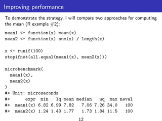
To demonstrate the strategy, I will compare two approaches for computing
the mean (R example #2):
mean1 <- function(x) mean(x)
mean2 <- function(x) sum(x) / length(x)
x <- runif(100)
stopifnot(all.equal(mean1(x), mean2(x)))
microbenchmark(
mean1(x),
mean2(x)
)
#> Unit: microseconds
#> expr min lq mean median uq max neval
#> mean1(x) 6.82 6.99 7.82 7.06 7.26 34.0 100
#> mean2(x) 1.24 1.40 1.77 1.73 1.84 11.5 100
12

Improving performance. Check for existing solutions
Has someone already solved the problem? Two good places to start are:
CRAN task views. If theres a CRAN task view related to your
problem domain, its worth looking at the packages listed there.
Reverse dependencies of Rcpp, as listed on its CRAN page. Since
these packages use C++, its possible to ﬁnd a solution to your
bottleneck written in a higher performance language.
13

Improving performance. Do as little as possible
The easiest way to make a function faster is to let it do less work. One
way to do that is use a function tailored to a more speciﬁc type of input
or output, or a more speciﬁc problem. For example:
rowSums(), colSums(), rowMeans(), and colMeans() are faster than
equivalent invocations that use apply() because they are vectorized
(the topic of the next section).
If you want to see if a vector contains a single value, any(x == 10) is
much faster than 10 %in% x. This is because testing equality is
simpler than testing inclusion in a set (R example #3).
14

Other functions will do less work if you give them more information
about the problem.
read.csv(): specify known column types with ’colClasses’
factor(): specify known levels with ’levels’ argument
cut(): don’t generate labels with labels = FALSE if you don’t need
them.
unlist(x, use.names = FALSE) is much faster than unlist(x) (R
example #4).
15

Sometimes you can make a function faster by avoiding method dispatch
which can be costly. If you are calling a method in a tight loop, you can
avoid some of the costs by doing the method lookup only once:
For S3, you can do this by calling generic.class() instead of generic().
For S4, you can do this by using ﬁndMethod() to ﬁnd the method,
saving it to a variable, and then calling that function.
For example, calling mean.default() is quite a bit faster than calling
mean() for small vectors (R example #5).
16

A ﬁnal example of doing less work is to use simpler data structures.
For example, when working with rows from a data frame, it is often faster
to work with row indices than data frames.
For instance, if you wanted to compute a bootstrap estimate of the
correlation between two columns in a data frame, there are two basic
approaches: you can either work with the whole data frame or with the
individual vectors. It can be shown that working with vectors is about
twice as fast (R example #6).
17

Improving performance. Vectorize
Vectorizing your code is not just about avoiding ”for” loops - it is about
taking a ”whole object” approach to a problem, thinking about vectors,
not scalars.
There are two key attributes of a vectorized function:
It makes many problems simpler. Instead of having to think about the
components of a vector, you only think about entire vectors.
The loops in a vectorized function are written in C instead of R.
Loops in C are much faster because they have much less overhead.
18

Vectorized functions that apply to many common performance bottlenecks
include:
rowSums(), colSums(), rowMeans(), and colMeans(). These
vectorised matrix functions will always be faster than using apply().
Vectorized subsetting - you can use subsetting assignment to replace
multiple values in a single step. If x is a vector, matrix or data frame
then x[is.na(x)] = 0 will replace all missing values with 0.
If you are extracting or replacing values in scattered locations in a
matrix or data frame, subset with an integer matrix (R example #7).
Be aware of vectorized functions like cumsum() and diﬀ () (R example
#8).
19

The downside of vectorization is that it makes it harder to predict how
operations will scale.
R example #9 - to look up 100 elements of a vector it only takes about 10
times longer(instead of a 100) than it does to look up 1 element.
And overall, it is often easier to write your own vectorized function in
C++ rather than torturing an existing algorithm into one that uses a
vectorized approach. You will learn how to do so in Rcpp.
20

Improving performance. Avoid copies
Avoiding copies is equivalent to avoiding growing an object with a
loop.
Whenever you use c(), append(), cbind(), rbind(), or paste() to create a
bigger object, R must:
ﬁrst allocate space for the new object
then copy the old object to its new home.
If you are repeating this many times, like in a ”for” loop, this can be quite
expensive.
R example #10: we will compare the operation of combining strings
iteratively with a loop(with a user-deﬁned function collapse()) against
doing it in a single pass(using paste()).
21

Improving performance. Byte code compilation
R 2.13.0 introduced a byte code compiler which can increase the speed
of some code with minimal eﬀort from your side.
The following example shows the pure R version of lapply() from the
”Functionals” chapter. Compiling it gives a considerable speedup,
although its still not quite as fast as the C version provided by base R (R
example #11).
lapply2 <- function(x, f, ...) {
out <- vector("list", length(x))
for (i in seq_along(x)) {
out[[i]] <- f(x[[i]], ...)
}
out
}

Improving performance. Byte code compilation
lapply2_c <- compiler::cmpfun(lapply2)
x <- list(1:10, letters, c(F, T), NULL)
microbenchmark(
lapply2(x, is.null),
lapply2_c(x, is.null),
lapply(x, is.null)
)
#> Unit: microseconds
#> expr min lq mean median uq max
#> lapply2(x, is.null) 9.92 11.30 13.42 11.80 12.40 49.2
#> lapply2_c(x, is.null) 4.40 5.18 5.79 5.53 5.83 15.1
#> lapply(x, is.null) 4.58 5.36 6.22 5.70 6.16 34.0
23

Improving performance. Case study: t-test
The following case study shows how to make t-tests faster using some
of the techniques described above (R example #12).
Imagine we have run 1000 experiments (rows), each of which collects data
on 50 individuals (columns). The ﬁrst 25 individuals in each experiment
are assigned to group 1 and the rest to group 2. We will ﬁrst generate
some random data to represent this problem:
m <- 1000
n <- 50
X <- matrix(rnorm(m * n, mean = 10, sd = 3), nrow = m)
grp <- rep(1:2, each = n / 2)

Speedup 1
For data in this form, there are two ways to use t.test():
using the formula interface
providing two vectors(one for each group).
Timing reveals that the formula interface is considerably slower.
system.time(for(i in 1:m) t.test(X[i, ] ~ grp)$stat)
#> user system elapsed
#> 1.4 0.0 1.4
system.time(
for(i in 1:m) t.test(X[i, grp == 1], X[i, grp == 2])$stat
)
#> 0.348 0.000 0.354
25

Of course, a for loop computes, but doesnt save the values - we will
use apply() to do that. This adds a little overhead:
compT <- function(x, grp){
t.test(x[grp == 1], x[grp == 2])$stat
}
system.time(t1 <- apply(X, 1, compT, grp = grp))
#> 0.341 0.000 0.341
26

Speedup 2
How can we make this faster? First, we could try doing less work.
Besides computing the t-statistic, stats :: t.test.default():
computes p-value
formats the output for printing
We can try to make our code faster by stripping out those pieces.
27

So we just write our own function:
my_t <- function(x, grp) {
t_stat <- function(x) {
m <- mean(x)
n <- length(x)
var <- sum((x - m) ^ 2) / (n - 1)
list(m = m, n = n, var = var)
}
g1 <- t_stat(x[grp == 1])
g2 <- t_stat(x[grp == 2])
se_total <- sqrt(g1$var / g1$n + g2$var / g2$n)
(g1$m - g2$m) / se_total
}

Checking its performance:
system.time(t2 <- apply(X, 1, my_t, grp = grp))
#> 0.049 0.000 0.049
stopifnot(all.equal(t1, t2))
This gives us about a 6x speed improvement.
29

Speedup 3
Now that we have a fairly simple function, we can make it faster still by
vectorizing it - modifying it to work with a matrix of values. Thus:
mean() becomes rowMeans()
length() becomes ncol()
sum() becomes rowSums()
the rest of the code stays the same.
30

After capturing above modiﬁcations in function rowtstat() we get:
system.time(t3 <- rowtstat(X, grp))
#> 0.003 0.000 0.003
stopifnot(all.equal(t1, t3))
Thats much faster! Its at least 40x faster than our previous eﬀort, and
around 1000x faster than where we started.
31

Improving performance. Parallelize
Parallelization uses multiple cores to work simultaneously on diﬀerent
parts of a problem. It saves your time because you are using more of your
computers resources.
Here we show application of parallel computing to what are called
”embarrassingly parallel problems” - ones made up of many simple
problems that can be solved independently.
Example - lapply() as it operates on each element independently of the
others.
Parallelizing lapply() on Linux and the Mac: substitute mclapply() for
lapply().
32

library(parallel)
cores <- detectCores()
cores
#> [1] 32
pause <- function(i) {
function(x) Sys.sleep(i)
}
system.time(lapply(1:10, pause(0.25)))
#> 0.002 0.000 2.504
system.time(mclapply(1:10, pause(0.25), mc.cores = cores))
#> 0.018 0.095 0.308

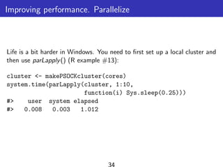
Life is a bit harder in Windows. You need to ﬁrst set up a local cluster and
then use parLapply() (R example #13):
cluster <- makePSOCKcluster(cores)
system.time(parLapply(cluster, 1:10,
function(i) Sys.sleep(0.25)))
#> 0.008 0.003 1.012
34

Other remarks
There is some communication overhead with parallel computing.
If the subproblems are very small, then parallelization might hurt
rather than help.
It is also possible to distribute computation over a network of
computers
35

Improving performance. Other techniques
Read R blogs to see what performance problems other people have
struggled with, and how they have made their code faster.
Read other R programming books, like Norm Matloff’s ”The Art of R
Programming” or Patrick Burns’ ”R Inferno” to learn about common
traps.
Take an algorithms and data structure course to learn some well
known ways of tackling certain classes of problems. I have heard good
things about Princetons Algorithms course offered on Coursera.
Read general books about optimization like ”Mature optimization” by
Carlos Bueno, or the ”Pragmatic Programmer” by Andrew Hunt and
David Thomas.
You can also reach out to the community for help. ”Stackoverflow”
can be a useful resource.
36

Oct.22nd.Presentation.Final

More Related Content

What's hot (20)

Viewers also liked (15)

Similar to Oct.22nd.Presentation.Final (20)

Oct.22nd.Presentation.Final