The document provides an overview of the Mundell-Fleming model, which examines how fiscal and monetary policy impact output and exchange rates under different exchange rate regimes. Key points:
1) Under floating exchange rates, fiscal policy has no effect on output while monetary policy is powerful. Under fixed rates, the reverse is true - fiscal policy is powerful while monetary policy has no effect.
2) A country cannot have free capital mobility, an independent monetary policy, and a fixed exchange rate at the same time. It must choose two of the three.
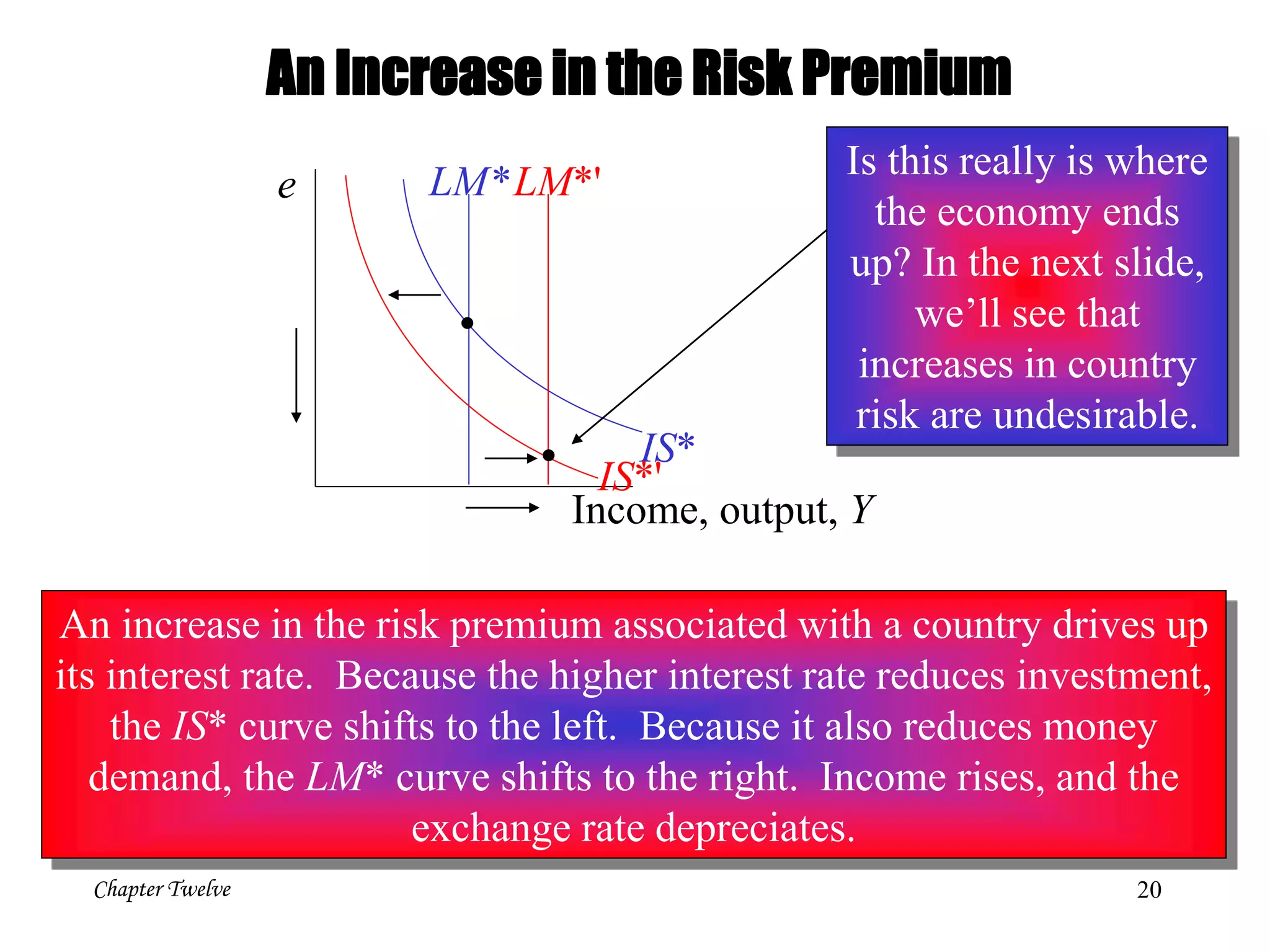
3) Expectations about exchange rate changes can become self-fulfilling prophecies that impact interest rates and currency values in the present. Increased risk perceptions push up


![[EM-Sofyan] Monopoly and Monopsony Market](https://cdn.slidesharecdn.com/ss_thumbnails/em-sofyanmonopolyandmonopsonymarket-140107174254-phpapp02-thumbnail.jpg?width=640&height=640&fit=bounds)


