SlideShare a Scribd company logo
Gradient Descent
Optimization Algorithms
Van Phu Quang Huy
Ta Duc Tung
Pham Quang Khang 1
Topics of today’s talk
● Function optimization
● Basics optimization algorithms and limitation
● Challenges in gradient descent optimization
● Practical gradient descent algorithms
2
Optimization in Machine learning
● Machine learning cares about performance measure P, that
is defined with respect to the test set and may also be
intractable
● Learning process: optimize P indirectly by optimizing a
cost function J(θ), in the hope that doing so will
improve P
● First problem of machine learning: optimization for cost
function J(θ)
3
Function Optimization
4
What is function optimization
● Optimization = minimizing or maximizing
● Maximizing a function f may be accomplished via
minimizing -f
● f is called an objective function or criterion
● In the case of minimization, f is also called cost
function, loss function, or error function
5
Optimization Problem
● Example: find extrema of function f(x,y)=x2
+y2
6
Optimization Problem
● Example: find extrema of function f(x,y)=x2
+y2
● Easy?
7
Optimization Problem
● Example: find extrema of function f(x,y)=x2
+y2
● Easy?
● How about f(x,y)=-x2
-y2
8
Optimization Problem
● Example: find extrema of function f(x,y)=x2
+y2
● Easy?
● How about f(x,y)=-x2
-y2
● Still easy?
9
Optimization Problem
● Example: find extrema of function f(x,y)=x2
+y2
● Easy?
● How about f(x,y)=-x2
-y2
● Still easy?
● How about f(x,y)=x2
-y2
10
Maxima, minima, and saddle points
11
f(x,y)=x2
+y2
f(x,y)=-x2
-y2
f(x,y)=x2
-y2
Gradient and the Hessian matrix
● Gradient: vector of first-order
partial derivatives
12
● Hessian: matrix of second-order
partial derivatives
Second Partial Derivative Test
f is a multivariate function
● Stationary points: points that make ∇f = 0
● Second partial derivative test:
A stationary point is
○ Local minimum if all eigenvalues of the Hessian positive
○ Local maximum if all eigenvalues of the Hessian negative
○ Saddle point if the Hessian has both positive and negative
eigenvalues
○ Inconclusive if the Hessian is invertible
13
Since H has 2 eigenvalues 1,3 > 0 then (0,0) is a minimum 14
Example: f(x,y) = x2
-xy+y2
Basic Optimization Algorithms
15
Batch Gradient Descent
Blindfolded Hiker: how to get to the lowest place?
16
θ*
: Position
What we need
to find
J(θ): Height
Batch Gradient Descent
Blindfolded Hiker: how to get to the lowest place?
17
Go step-by-step
● Which direction?
Left or Right?
● How far should I step?
Gradient
Learning
Rate
Batch Gradient Descent
Solution: θ := θ - η∇θ
J(θ)
1. Initiate step size η
2. Start with a random point θ
3. Calculate gradient ∇θ
J(θ) at point θ
4. Follow the inversed direction of gradient → get new θ
5. Repeat until reach minima
a. Stop condition? → gradient is small enough
18
Batch Gradient Descent
Pros
● Stable convergence
Cons
● Need to calculate gradient for whole dataset
● Slow if is not implemented wisely
19
Stochastic Gradient Descent
Principle: Same as Batch Gradient Descent
Difference:
● Updating θ at each example of training dataset
20
θ := θ - η∇θ
J(θ)
θ := θ - η∇θ
J(θ;x(i)
,y(i)
)
Stochastic Gradient Descent
Pros
● Faster than Batch Gradient
● Possible to learn online
Cons
● Unstable convergence
● Not use optimized vector operation
21
Image Credit: Pham Quang Khang
Fluctuation in Stochastic Gradient Descent
Optimization in Machine Learning
22
Example of a cost function
● Example: cross entropy in logistic regression
where xn
is vector input, yn
is label, w is weight matrix, N
is number of training examples, σ is sigmoid function
● The shape of the cost function is poorly understood
23
Convexity problem
● In traditional machine learning, objective functions are
designed carefully to be convex
○ Example: objective function of SVM is convex.
● When training neural networks, we must confront the
non-convex case
○ Many local minima → infeasible to find global minima
○ Dealing with saddle points
○ Flat regions exist
24
Local minima
● In practice, local minima is not a major problem
● [1] gives some theoretical insights about local minima:
○ For large-size networks, most local minima are equivalent and yield
similar performance on a test set
○ The probability of finding a “bad” (high value) local minimum is
non-zero for small-size networks and decreases quickly with network
size
○ Struggling to find the global minimum on the training set (as opposed
to one of the many good local ones) is not useful in practice and may
lead to overfitting
25[1] Choromanska et al. 2014.
Saddle points
● For high-dimensional non-convex functions, saddle points
are much more than local minima (and maxima) [1]
● Saddle points slow down training process
○ Batch Gradient Descent may be stuck at saddle points
○ Stochastic Gradient Descent seems to be able to escape saddle points
in many cases [2]
26
[1] Dauphin et al. 2014.
[2] Goodfellow et al. 2015.
Flat regions
● Flat regions: regions of constant value, where the
gradient and the Hessian are both 0
● Big problem when those regions have high value of the
objective function
● Escaping from those regions is extremely difficult
27y = x5
● At (0,0) the gradient and the
Hessian are both 0
→ f is super flat at (0,0)
● Second partial derivative test
can’t determine whether (0,0)
is a local minimum, a local
maximum or a saddle point
● In this case, (0,0) is a
global maximum
28
Flat regions: example of cost function f(x,y) = -x2
y2
Flat regions: example of cost function f(x,y) = xy(x+y)(1+y)
● At (0,0) the gradient and the
Hessian are both 0 too
● But in this case, (0,0) is a
saddle point
29
Practical Gradient Descent Algorithms
30
Gradient descent optimization problem
● Objective: to find the parameters θ that minimize the
lost function J(θ)
● Approach: iteratively update the params θ by utilizing
the gradient ∇J(θ)
● Gradient descent conventional method: θt
= θt-1
- η∇J(θ)
31
Momentum
● Add momentum to params updater:
vt
= αvt-1
- η∇J(θt-1
)
θt
= θt-1
+ vt
● Essential meaning of Momentum:
○ Accelerate the learning rate during the training process
○ In physic: add the momentum to the ball that rolling down the hill
○ The momentum parameter α is less than 1 as there is always resistance
force to slow the ball down and usually picked as 0.9
32
Adaptive learning rate
● Previous algorithm always use the fixed learning rate
throughout the learning process
○ The learning rate has to be either set to be very small at the
beginning or periodically decrease the learning rate
● Adaptive learning rate: learning rate is automatically
decreased in the learning process
● Adaptive learning rate algo: AdaGrad, RMSprop, Adam
33
Adagrad
● Essential meaning: the larger the params change the
slower it get updated
● Algorithms:
Accumulated sum-square ht
= ht-1
+ ∇J(θt-1
)・∇J(θt-1
)
Params updater θt
= θt-1
- η(1/sqrt(ht
))・∇J(θ)
● The learning rate is decreased as the number of update
step increases
34
RMSprop
● Adagrad decreases the learning rate too fast as it adds
all previous square gradients
● Consider partially previous added up sum square gradient:
Accumulated sum-square ht
= γht-1
+ (1-γ)∇J(θt-1
)・∇J(θt-1
)
Params updater θt
= θt-1
- η(1/sqrt(ht
))・∇J(θt-1
)
● Good practice γ = 0.9
35
Adam (Adaptive momentum estimation)
● Utilizing the advantage of both Momentum and Adagrad
● Algorithm
Momentum: vt
= β1
vt-1
+ (1 - β1
)∇J(θt-1
)
Learning rate: ht
= β2
ht-1
+ (1 - β2
)∇J(θt-1
)・∇J(θt-1
)
To avoid momentum and learning rate decay to be too
small, zero-bias counteract is calculated:
Vt
’ = vt
/(1 - β1
t
), ht
’ = ht
/(1 - β2
t
)
Param update:
θt
= θt-1
- ηVt
’/(sqrt(ht
’) + ε)
36
Compare all 4 algorithms +SGD on benchmark data
● Data: part of MNIST
● Input size: 28x28x1, output size: 10
● Model: NN with 4 hidden layers, 100 units each layer
● Train data number: 800, test data number: 200
● Batch size: 100
● Number of epoch: 1000
● Initial weight: Ɲ(0, 0.1)
37
Result 1: Change of cost function during process
● Learning rate: η = 0.001
● Momentum: α = 0.9
● RMSprop: γ = 0.9
● Adam: β1
= 0.9, β2
= 0.999
38
Result 2: Accuracy of training
Training set
39
Test set
Simple CNN test
● Conv - pool - fully connected - softmax
● Conv params:
○ Filter number: 30
○ Filter size: 5x5x1
○ Pad: 0
○ Stride: 1
● Input size: 28x28x1, output size: 10
● Train data: 800, test: 200
● Number epoch: 50
● FC layer size: 100
40
Simple CNN result1: cost function
● Learning rate: η = 0.001
● Momentum: α = 0.9
● RMSProp: γ = 0.9
● Adam: β1
= 0.9, β2
= 0.999
41
Simple CNN result 2: accuracy
Train
42
Test
References
43
Machine Learning Definition
"A computer program is said to learn from experience E with
respect to some class of tasks T and performance measure P
if its performance at tasks in T, as measured by P, improves
with experience E." [1]
[1] Mitchell, T. (1997). Machine Learning. McGraw Hill. p2.
44
Exploding Gradients
● Cliffs: where the
gradient is super big
● One update step of
gradient descent can
move the parameters
extremely far, usually
over the minimum point
● Solution: gradient
clipping
45
Goodfellow et al, Deep Learning book, p289
Vanishing Gradients
● Is a major problem when training deep networks
● The gradient tends to get smaller as we move backward
through the hidden layers when running backpropagation
● Weights in the earlier layers may not be learned
● Solutions:
○ Use good activation functions (e.g. ReLU) instead of sigmoid
○ Good initialization
○ Better network architectures (LSTMs/GRUs instead of basic RNNs)
46
Sharp and Wide Minima [1]
● Large-batch Gradient Descent tends to converge to sharp minima
→ poorer generalization
● Small-batch Gradient Descent consistently converges to wide minima
→ better generalization
47[1] Keskar et al. 2017.

More Related Content

What's hot (20)

PDF
Convolutional Neural Networks : Popular Architectures
ananth
 
PDF
Training Neural Networks
Databricks
 
PDF
Methods of Optimization in Machine Learning
Knoldus Inc.
 
PDF
Transfer Learning
Hichem Felouat
 
PDF
Gradient descent method
Sanghyuk Chun
 
PPTX
Hyperparameter Tuning
Jon Lederman
 
PPTX
An overview of gradient descent optimization algorithms
Hakky St
 
PPTX
Deep Neural Networks (DNN)
Sir Syed University of Engineering & Technology
 
PPTX
Soft computing
ganeshpaul6
 
PPTX
04 Multi-layer Feedforward Networks
Tamer Ahmed Farrag, PhD
 
PPTX
Optimization problems and algorithms
Aboul Ella Hassanien
 
PDF
Nature-Inspired Optimization Algorithms
Xin-She Yang
 
PPTX
Self-organizing map
Tarat Diloksawatdikul
 
PPTX
CNN Tutorial
Sungjoon Choi
 
PPTX
Multilayer Perceptron Neural Network MLP
Abdullah al Mamun
 
PPTX
Regularization in deep learning
Kien Le
 
PPTX
Basics of Soft Computing
Sangeetha Rajesh
 
PPT
Genetic Algorithms - Artificial Intelligence
Sahil Kumar
 
PPT
Feature Extraction and Principal Component Analysis
Sayed Abulhasan Quadri
 
PPT
Introduction to soft computing
Ankush Kumar
 
Convolutional Neural Networks : Popular Architectures
ananth
 
Training Neural Networks
Databricks
 
Methods of Optimization in Machine Learning
Knoldus Inc.
 
Transfer Learning
Hichem Felouat
 
Gradient descent method
Sanghyuk Chun
 
Hyperparameter Tuning
Jon Lederman
 
An overview of gradient descent optimization algorithms
Hakky St
 
Soft computing
ganeshpaul6
 
04 Multi-layer Feedforward Networks
Tamer Ahmed Farrag, PhD
 
Optimization problems and algorithms
Aboul Ella Hassanien
 
Nature-Inspired Optimization Algorithms
Xin-She Yang
 
Self-organizing map
Tarat Diloksawatdikul
 
CNN Tutorial
Sungjoon Choi
 
Multilayer Perceptron Neural Network MLP
Abdullah al Mamun
 
Regularization in deep learning
Kien Le
 
Basics of Soft Computing
Sangeetha Rajesh
 
Genetic Algorithms - Artificial Intelligence
Sahil Kumar
 
Feature Extraction and Principal Component Analysis
Sayed Abulhasan Quadri
 
Introduction to soft computing
Ankush Kumar
 

Similar to Overview on Optimization algorithms in Deep Learning (20)

PPTX
Deep Neural Network Module 3A Optimization.pptx
ratnababum
 
PDF
Dep Neural Networks introduction new.pdf
ratnababum
 
PDF
Regresssion technique part of Machine learning
sstouqeer425
 
PDF
Gradient_Descent_Unconstrained.pdf
MTrang34
 
PDF
4optmizationtechniques-150308051251-conversion-gate01.pdf
BechanYadav4
 
PPTX
Optmization techniques
Deepshika Reddy
 
PDF
optmizationtechniques.pdf
SantiagoGarridoBulln
 
PPTX
Optimization of mathematical function using gradient descent algorithm.pptx
s17714274
 
PPTX
super vector machines algorithms using deep
KNaveenKumarECE
 
PDF
Regression_1.pdf
Amir Saleh
 
PDF
MUMS: Transition & SPUQ Workshop - Practical Bayesian Optimization for Urban ...
The Statistical and Applied Mathematical Sciences Institute
 
PPTX
daa-unit-3-greedy method
hodcsencet
 
PPTX
Lec2-review-III-svm-logreg_for the beginner.pptx
raheemsyedrameez12
 
PDF
Machine learning using matlab.pdf
ppvijith
 
PDF
final-ppts-daa-unit-iii-greedy-method.pdf
JasmineSayyed3
 
PDF
Introduction to Artificial Neural Networks
Stratio
 
PDF
Program on Quasi-Monte Carlo and High-Dimensional Sampling Methods for Applie...
The Statistical and Applied Mathematical Sciences Institute
 
PDF
Combinatorial optimization CO-1
man003
 
PDF
Paper Study: Melding the data decision pipeline
ChenYiHuang5
 
PPTX
Optimization tutorial
Northwestern University
 
Deep Neural Network Module 3A Optimization.pptx
ratnababum
 
Dep Neural Networks introduction new.pdf
ratnababum
 
Regresssion technique part of Machine learning
sstouqeer425
 
Gradient_Descent_Unconstrained.pdf
MTrang34
 
4optmizationtechniques-150308051251-conversion-gate01.pdf
BechanYadav4
 
Optmization techniques
Deepshika Reddy
 
optmizationtechniques.pdf
SantiagoGarridoBulln
 
Optimization of mathematical function using gradient descent algorithm.pptx
s17714274
 
super vector machines algorithms using deep
KNaveenKumarECE
 
Regression_1.pdf
Amir Saleh
 
MUMS: Transition & SPUQ Workshop - Practical Bayesian Optimization for Urban ...
The Statistical and Applied Mathematical Sciences Institute
 
daa-unit-3-greedy method
hodcsencet
 
Lec2-review-III-svm-logreg_for the beginner.pptx
raheemsyedrameez12
 
Machine learning using matlab.pdf
ppvijith
 
final-ppts-daa-unit-iii-greedy-method.pdf
JasmineSayyed3
 
Introduction to Artificial Neural Networks
Stratio
 
Program on Quasi-Monte Carlo and High-Dimensional Sampling Methods for Applie...
The Statistical and Applied Mathematical Sciences Institute
 
Combinatorial optimization CO-1
man003
 
Paper Study: Melding the data decision pipeline
ChenYiHuang5
 
Optimization tutorial
Northwestern University
 
Ad

Recently uploaded (20)

PDF
apidays Singapore 2025 - From API Intelligence to API Governance by Harsha Ch...
apidays
 
PDF
apidays Helsinki & North 2025 - Monetizing AI APIs: The New API Economy, Alla...
apidays
 
PDF
OPPOTUS - Malaysias on Malaysia 1Q2025.pdf
Oppotus
 
PDF
JavaScript - Good or Bad? Tips for Google Tag Manager
📊 Markus Baersch
 
PPTX
apidays Singapore 2025 - Designing for Change, Julie Schiller (Google)
apidays
 
PPTX
Exploring Multilingual Embeddings for Italian Semantic Search: A Pretrained a...
Sease
 
PDF
Simplifying Document Processing with Docling for AI Applications.pdf
Tamanna
 
PDF
apidays Helsinki & North 2025 - How (not) to run a Graphql Stewardship Group,...
apidays
 
PPTX
apidays Singapore 2025 - The Quest for the Greenest LLM , Jean Philippe Ehre...
apidays
 
PPTX
apidays Munich 2025 - Building Telco-Aware Apps with Open Gateway APIs, Subhr...
apidays
 
PPTX
Numbers of a nation: how we estimate population statistics | Accessible slides
Office for National Statistics
 
PPTX
Listify-Intelligent-Voice-to-Catalog-Agent.pptx
nareshkottees
 
PDF
apidays Singapore 2025 - How APIs can make - or break - trust in your AI by S...
apidays
 
PPT
AI Future trends and opportunities_oct7v1.ppt
SHIKHAKMEHTA
 
PPTX
SlideEgg_501298-Agentic AI.pptx agentic ai
530BYManoj
 
PDF
What does good look like - CRAP Brighton 8 July 2025
Jan Kierzyk
 
PPTX
apidays Helsinki & North 2025 - Agentic AI: A Friend or Foe?, Merja Kajava (A...
apidays
 
PDF
apidays Singapore 2025 - Building a Federated Future, Alex Szomora (GSMA)
apidays
 
PDF
apidays Singapore 2025 - Surviving an interconnected world with API governanc...
apidays
 
PDF
Context Engineering for AI Agents, approaches, memories.pdf
Tamanna
 
apidays Singapore 2025 - From API Intelligence to API Governance by Harsha Ch...
apidays
 
apidays Helsinki & North 2025 - Monetizing AI APIs: The New API Economy, Alla...
apidays
 
OPPOTUS - Malaysias on Malaysia 1Q2025.pdf
Oppotus
 
JavaScript - Good or Bad? Tips for Google Tag Manager
📊 Markus Baersch
 
apidays Singapore 2025 - Designing for Change, Julie Schiller (Google)
apidays
 
Exploring Multilingual Embeddings for Italian Semantic Search: A Pretrained a...
Sease
 
Simplifying Document Processing with Docling for AI Applications.pdf
Tamanna
 
apidays Helsinki & North 2025 - How (not) to run a Graphql Stewardship Group,...
apidays
 
apidays Singapore 2025 - The Quest for the Greenest LLM , Jean Philippe Ehre...
apidays
 
apidays Munich 2025 - Building Telco-Aware Apps with Open Gateway APIs, Subhr...
apidays
 
Numbers of a nation: how we estimate population statistics | Accessible slides
Office for National Statistics
 
Listify-Intelligent-Voice-to-Catalog-Agent.pptx
nareshkottees
 
apidays Singapore 2025 - How APIs can make - or break - trust in your AI by S...
apidays
 
AI Future trends and opportunities_oct7v1.ppt
SHIKHAKMEHTA
 
SlideEgg_501298-Agentic AI.pptx agentic ai
530BYManoj
 
What does good look like - CRAP Brighton 8 July 2025
Jan Kierzyk
 
apidays Helsinki & North 2025 - Agentic AI: A Friend or Foe?, Merja Kajava (A...
apidays
 
apidays Singapore 2025 - Building a Federated Future, Alex Szomora (GSMA)
apidays
 
apidays Singapore 2025 - Surviving an interconnected world with API governanc...
apidays
 
Context Engineering for AI Agents, approaches, memories.pdf
Tamanna
 
Ad

Overview on Optimization algorithms in Deep Learning

  • 1. Gradient Descent Optimization Algorithms Van Phu Quang Huy Ta Duc Tung Pham Quang Khang 1
  • 2. Topics of today’s talk ● Function optimization ● Basics optimization algorithms and limitation ● Challenges in gradient descent optimization ● Practical gradient descent algorithms 2
  • 3. Optimization in Machine learning ● Machine learning cares about performance measure P, that is defined with respect to the test set and may also be intractable ● Learning process: optimize P indirectly by optimizing a cost function J(θ), in the hope that doing so will improve P ● First problem of machine learning: optimization for cost function J(θ) 3
  • 5. What is function optimization ● Optimization = minimizing or maximizing ● Maximizing a function f may be accomplished via minimizing -f ● f is called an objective function or criterion ● In the case of minimization, f is also called cost function, loss function, or error function 5
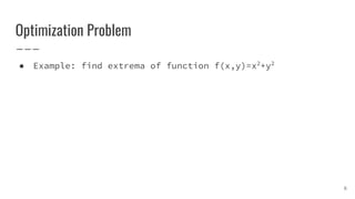
  • 6. Optimization Problem ● Example: find extrema of function f(x,y)=x2 +y2 6
  • 7. Optimization Problem ● Example: find extrema of function f(x,y)=x2 +y2 ● Easy? 7
  • 8. Optimization Problem ● Example: find extrema of function f(x,y)=x2 +y2 ● Easy? ● How about f(x,y)=-x2 -y2 8
  • 9. Optimization Problem ● Example: find extrema of function f(x,y)=x2 +y2 ● Easy? ● How about f(x,y)=-x2 -y2 ● Still easy? 9
  • 10. Optimization Problem ● Example: find extrema of function f(x,y)=x2 +y2 ● Easy? ● How about f(x,y)=-x2 -y2 ● Still easy? ● How about f(x,y)=x2 -y2 10
  • 11. Maxima, minima, and saddle points 11 f(x,y)=x2 +y2 f(x,y)=-x2 -y2 f(x,y)=x2 -y2
  • 12. Gradient and the Hessian matrix ● Gradient: vector of first-order partial derivatives 12 ● Hessian: matrix of second-order partial derivatives
  • 13. Second Partial Derivative Test f is a multivariate function ● Stationary points: points that make ∇f = 0 ● Second partial derivative test: A stationary point is ○ Local minimum if all eigenvalues of the Hessian positive ○ Local maximum if all eigenvalues of the Hessian negative ○ Saddle point if the Hessian has both positive and negative eigenvalues ○ Inconclusive if the Hessian is invertible 13
  • 14. Since H has 2 eigenvalues 1,3 > 0 then (0,0) is a minimum 14 Example: f(x,y) = x2 -xy+y2
  • 16. Batch Gradient Descent Blindfolded Hiker: how to get to the lowest place? 16 θ* : Position What we need to find J(θ): Height
  • 17. Batch Gradient Descent Blindfolded Hiker: how to get to the lowest place? 17 Go step-by-step ● Which direction? Left or Right? ● How far should I step? Gradient Learning Rate
  • 18. Batch Gradient Descent Solution: θ := θ - η∇θ J(θ) 1. Initiate step size η 2. Start with a random point θ 3. Calculate gradient ∇θ J(θ) at point θ 4. Follow the inversed direction of gradient → get new θ 5. Repeat until reach minima a. Stop condition? → gradient is small enough 18
  • 19. Batch Gradient Descent Pros ● Stable convergence Cons ● Need to calculate gradient for whole dataset ● Slow if is not implemented wisely 19
  • 20. Stochastic Gradient Descent Principle: Same as Batch Gradient Descent Difference: ● Updating θ at each example of training dataset 20 θ := θ - η∇θ J(θ) θ := θ - η∇θ J(θ;x(i) ,y(i) )
  • 21. Stochastic Gradient Descent Pros ● Faster than Batch Gradient ● Possible to learn online Cons ● Unstable convergence ● Not use optimized vector operation 21 Image Credit: Pham Quang Khang Fluctuation in Stochastic Gradient Descent
  • 22. Optimization in Machine Learning 22
  • 23. Example of a cost function ● Example: cross entropy in logistic regression where xn is vector input, yn is label, w is weight matrix, N is number of training examples, σ is sigmoid function ● The shape of the cost function is poorly understood 23
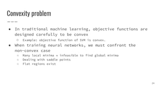
  • 24. Convexity problem ● In traditional machine learning, objective functions are designed carefully to be convex ○ Example: objective function of SVM is convex. ● When training neural networks, we must confront the non-convex case ○ Many local minima → infeasible to find global minima ○ Dealing with saddle points ○ Flat regions exist 24
  • 25. Local minima ● In practice, local minima is not a major problem ● [1] gives some theoretical insights about local minima: ○ For large-size networks, most local minima are equivalent and yield similar performance on a test set ○ The probability of finding a “bad” (high value) local minimum is non-zero for small-size networks and decreases quickly with network size ○ Struggling to find the global minimum on the training set (as opposed to one of the many good local ones) is not useful in practice and may lead to overfitting 25[1] Choromanska et al. 2014.
  • 26. Saddle points ● For high-dimensional non-convex functions, saddle points are much more than local minima (and maxima) [1] ● Saddle points slow down training process ○ Batch Gradient Descent may be stuck at saddle points ○ Stochastic Gradient Descent seems to be able to escape saddle points in many cases [2] 26 [1] Dauphin et al. 2014. [2] Goodfellow et al. 2015.
  • 27. Flat regions ● Flat regions: regions of constant value, where the gradient and the Hessian are both 0 ● Big problem when those regions have high value of the objective function ● Escaping from those regions is extremely difficult 27y = x5
  • 28. ● At (0,0) the gradient and the Hessian are both 0 → f is super flat at (0,0) ● Second partial derivative test can’t determine whether (0,0) is a local minimum, a local maximum or a saddle point ● In this case, (0,0) is a global maximum 28 Flat regions: example of cost function f(x,y) = -x2 y2
  • 29. Flat regions: example of cost function f(x,y) = xy(x+y)(1+y) ● At (0,0) the gradient and the Hessian are both 0 too ● But in this case, (0,0) is a saddle point 29
  • 30. Practical Gradient Descent Algorithms 30
  • 31. Gradient descent optimization problem ● Objective: to find the parameters θ that minimize the lost function J(θ) ● Approach: iteratively update the params θ by utilizing the gradient ∇J(θ) ● Gradient descent conventional method: θt = θt-1 - η∇J(θ) 31
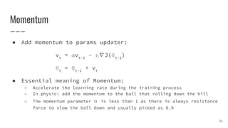
  • 32. Momentum ● Add momentum to params updater: vt = αvt-1 - η∇J(θt-1 ) θt = θt-1 + vt ● Essential meaning of Momentum: ○ Accelerate the learning rate during the training process ○ In physic: add the momentum to the ball that rolling down the hill ○ The momentum parameter α is less than 1 as there is always resistance force to slow the ball down and usually picked as 0.9 32
  • 33. Adaptive learning rate ● Previous algorithm always use the fixed learning rate throughout the learning process ○ The learning rate has to be either set to be very small at the beginning or periodically decrease the learning rate ● Adaptive learning rate: learning rate is automatically decreased in the learning process ● Adaptive learning rate algo: AdaGrad, RMSprop, Adam 33
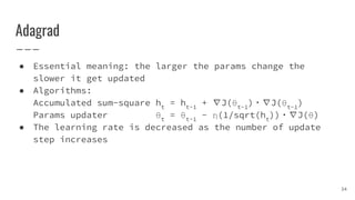
  • 34. Adagrad ● Essential meaning: the larger the params change the slower it get updated ● Algorithms: Accumulated sum-square ht = ht-1 + ∇J(θt-1 )・∇J(θt-1 ) Params updater θt = θt-1 - η(1/sqrt(ht ))・∇J(θ) ● The learning rate is decreased as the number of update step increases 34
  • 35. RMSprop ● Adagrad decreases the learning rate too fast as it adds all previous square gradients ● Consider partially previous added up sum square gradient: Accumulated sum-square ht = γht-1 + (1-γ)∇J(θt-1 )・∇J(θt-1 ) Params updater θt = θt-1 - η(1/sqrt(ht ))・∇J(θt-1 ) ● Good practice γ = 0.9 35
  • 36. Adam (Adaptive momentum estimation) ● Utilizing the advantage of both Momentum and Adagrad ● Algorithm Momentum: vt = β1 vt-1 + (1 - β1 )∇J(θt-1 ) Learning rate: ht = β2 ht-1 + (1 - β2 )∇J(θt-1 )・∇J(θt-1 ) To avoid momentum and learning rate decay to be too small, zero-bias counteract is calculated: Vt ’ = vt /(1 - β1 t ), ht ’ = ht /(1 - β2 t ) Param update: θt = θt-1 - ηVt ’/(sqrt(ht ’) + ε) 36
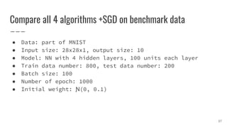
  • 37. Compare all 4 algorithms +SGD on benchmark data ● Data: part of MNIST ● Input size: 28x28x1, output size: 10 ● Model: NN with 4 hidden layers, 100 units each layer ● Train data number: 800, test data number: 200 ● Batch size: 100 ● Number of epoch: 1000 ● Initial weight: Ɲ(0, 0.1) 37
  • 38. Result 1: Change of cost function during process ● Learning rate: η = 0.001 ● Momentum: α = 0.9 ● RMSprop: γ = 0.9 ● Adam: β1 = 0.9, β2 = 0.999 38
  • 39. Result 2: Accuracy of training Training set 39 Test set
  • 40. Simple CNN test ● Conv - pool - fully connected - softmax ● Conv params: ○ Filter number: 30 ○ Filter size: 5x5x1 ○ Pad: 0 ○ Stride: 1 ● Input size: 28x28x1, output size: 10 ● Train data: 800, test: 200 ● Number epoch: 50 ● FC layer size: 100 40
  • 41. Simple CNN result1: cost function ● Learning rate: η = 0.001 ● Momentum: α = 0.9 ● RMSProp: γ = 0.9 ● Adam: β1 = 0.9, β2 = 0.999 41
  • 42. Simple CNN result 2: accuracy Train 42 Test
  • 44. Machine Learning Definition "A computer program is said to learn from experience E with respect to some class of tasks T and performance measure P if its performance at tasks in T, as measured by P, improves with experience E." [1] [1] Mitchell, T. (1997). Machine Learning. McGraw Hill. p2. 44
  • 45. Exploding Gradients ● Cliffs: where the gradient is super big ● One update step of gradient descent can move the parameters extremely far, usually over the minimum point ● Solution: gradient clipping 45 Goodfellow et al, Deep Learning book, p289
  • 46. Vanishing Gradients ● Is a major problem when training deep networks ● The gradient tends to get smaller as we move backward through the hidden layers when running backpropagation ● Weights in the earlier layers may not be learned ● Solutions: ○ Use good activation functions (e.g. ReLU) instead of sigmoid ○ Good initialization ○ Better network architectures (LSTMs/GRUs instead of basic RNNs) 46
  • 47. Sharp and Wide Minima [1] ● Large-batch Gradient Descent tends to converge to sharp minima → poorer generalization ● Small-batch Gradient Descent consistently converges to wide minima → better generalization 47[1] Keskar et al. 2017.