SlideShare a Scribd company logo
Principal Component Analysis (PCA) –
In vs. Out of Model
1
Rodolfo J. Romañach, Ph.D.
QUIM 6835 Chemometrcs
February 23, 2022
“a database is not a vault, it is a
garden.“
Rene Marie Pacella
2
Scores Provide a
MAP of Samples
Loadings Provide a
MAP of Variable
Interrelationships
Esbensen KH (2012)
Multivariate Data
Analysis- in practice.
5th edn. CAMO
Software, page 44.
Scores cannot be
interpreted without
loadings; loadings
cannot be interpreted
without scores.
“Loadings describe the
data structure in terms
of variable contributions
and correlations. Every
variable analyzed has a
loading on each PC,
which reflects how much
the individual variable
contributes to that
PC, and how well the PC
takes into account the
variation contained in a
variable.”
Loadings Score Plots
Loadings Line Plots
“Loadings describe the
data structure in terms
of variable contributions
and correlations. Every
variable analyzed has a
loading on each PC,
which reflects how much
the individual variable
contributes to that
PC, and how well the PC
takes into account the
variation contained in a
variable.”
Loadings
• Loadings – map of variables.
• “The PCs are in fact nothing but linear combinations
of the original variables (unit vectors). Returning to a
previous definition, the loadings provide a “weighting”
of each variable’s contribution to a PC direction. When
a weighting is high for a variable, i.e. the variable has
a high loading (numerically), this variable contributes
significantly to the variance expressed by that PC.”
• X = TPT + E
• TPT describes the model. E is not the model, it is the
residual variation that is not included in the model.
Esbensen, K. E.; Swarbrick, B., Multivariate Data Analysis – in practice. An Introduction.
6th ed.; IMPublishing: 2018. page 78.
 If the spectral noise is known to be 0.1%, then how many
principal components should be used to explain the data ?
 Here we have the opportunity to filter or reduce the spectral
noise since we do not have to keep the eight factors.
Principal Components Analysis (PCA)
Principal Component Analysis
• X = TPT + E
• TPT describes the model. E is not the model, it is the
residual variation that is not included in the model.
• This is a description of PCA, but more importantly it
follows:
Data structure is correlated with the property of interest,
while noise is everything else, such as instrumental noise
(high frequency, low frequency noise, etc). Noise is what
is not included within the model (data structure) –
unexplained
Esbensen KH (2012) Multivariate Data Analysis- in practice. 5th
edn. CAMO Software,
95% Confidence Interval
The distance from the multivariate mean, commonly referred to as the
Mahalanobis distance (MD), is computed with the scores. In Hotelling’s T2 test,
the squared MD values are called Hotelling’s T2 values which are compared with
a table of critical values.
De Maesschalck, R.; Jouan-Rimbaud, D.; Massart, D. L., The Mahalanobis
distance. Chemometrics Intellig. Lab. Syst. 2000, 50 (1), 1-18.
Understanding Hotelling’s T2 Test
• In univariate statistics the t-test is used to
estimate confidence interval for one variable.
• This is the estimation of confidence interval for
a multivariate system.
• Confidence limits are built using the training
set which would contain measurements that
represent the normal (in control) situation.
• The computed MD (the so-called T2 value) of
each value is compared to a critical T2 value.
• Used to build multivariate process control
charts using the original variables or PCs.
Euclidean & Mahalonobis Distance
The Euclidean distance would tell us the distance
traveled.
However, if there is bad weather or there are many
airplanes trying to land the distance traveled would
be greater. The distance traveled would not be the
same for every flight. In that case we could
calculate a Mahalanobis distance based on the
standard deviations of the actual travel distances.
The Mahalanobis distance is thus a statistical
distance.
Projection of Samples Into Model
• Once the PCA model is developed you can project
samples into this model.
• “Projection is the method of taking a new object
and “transforming” it through the loadings of an
existing model to produce a new score value in
multivariate space.”-Esbensen page 151.
• “a new object can be projected onto an existing
model and the position of the new object can be
determined as being part of the model population,
or as being distinctly different. Esbensen page 151”
Esbensen, K. E.; Swarbrick, B., Multivariate Data Analysis – in practice.
An Introduction. 6th ed.; IMPublishing: 2018.
PCA Score Plot
The calibration set (Red points, 0-14.46 %w/w) was
used to predict blends of 20% w/w with a different API
(Blue) and excipients under the same spectral
acquisition parameters. These are outside the 95% CI
of model.
What are Outliers?
• Outliers are unusual samples that have a different
pattern that the rest of the samples, and could require
an extra factor to describe them. – Pirouette
• “Any observation that does not fit a pattern” - Miller
• Outliers may be measurement errors, for example
when there is no sample in front of Raman or NIR
probe, and it just sees air.
• “Some packages include elaborate diagnostics for so-
called outliers, which may in many cases be perfectly
good samples but ones whose correlation structure
differs from that of the training set.” - Brereton
Pirouette Manual, page 5-23 .
Chemometrics. Data Analysis for the Laboratory and Chemical Plant. Richard G. Brereton,
Wiley, 2003, Page 72.
Miller, Chemometrics in Process Analytical Chemistry.
14
PCA and outliers
• PCA is a good tool for visualization of outliers in
the X data. Visualizing spectra or samples that do
not follow the same pattern as the rest.
• If a sample’s score is separated from others it may
be an outlier. We may not know the reason for the
outlier, but if we pin-point it that’s a start. Later on
we can determine a physical or chemical reason for
the outlier.
• The score and error contributes indicate which
variables may cause the sample to be different.
• PCA model can be used as a benchmark for future
samples.
Pirouette Manual. 5-14, and 5-19. Infometrix.
15
In Model vs. Out of Model
In-Model vs. Out of Model
• Hotelling’s T2 test indicates whether a sample
is an outlier based on scores (variation
captured by model).
• The X-residuals provides an “out of model” –
assessment of outliers. The Q statistic flags
samples with unusual outliers.
• These are two complementary views, and
often used in real time process measurements.
17
Pirouette Manual 4.02, Infometrix, page 5-25
*- The Q statistic is also referred to as the square prediction error (squared
residual variance) . The value of Q can be obtained from its approximate
distribution. Pirouette manual 5-24.
Real Time Latent Variable Predictor
YES
Spectrum
similar to
calib.model
predict
blend conc.
Other calib model
Outlier
(inst. malfunction
or
process change)
Analytical methods are not applicable to all
materials, they are applicable to a certain
formulation or product. First test with PCA
determines applicability of method.
Process Control Application – using the Calib.
Model
Control hardware and software integration
Computers and Chemical Engineering 66 (2014) 186–200
Step 2 – Method for RT analysis
Step 3 –
sensors
integrated
into plant
Step 4 –
signal to
Control
platform
Step 1 -
Design
Industrial Application
• Software like SIMCA, Unscrambler, Pirouette, PLS
Tool Box, PLS IQ, etc are used to develop the
calibration model.
• This is another software that is just for “use” of
the calibration model and provide the information
to a distributed control system or plant
manufacturing data system.
• A number of companies sell software for real time
predictions. Software that enable the use of the
regression equation in the production
environment.
• Significant opportunity for quality improvement
and process knowledge.
Principal Component Analysis (PCA) –
In vs. Out of Model – Importance of
Residuals
22
Rodolfo J. Romañach, Ph.D.
QUIM 6835 Chemometrcs
March 4, 2022
Projection of Samples Into Model
• Use an existing model to predict unknown samples.
• Once the PCA model is developed you can project
samples into this model.
• “Projection is the method of taking a new object
and “transforming” it through the loadings of an
existing model to produce a new score value in
multivariate space.”-Esbensen page 151.
• “a new object can be projected onto an existing
model and the position of the new object can be
determined as being part of the model population,
or as being distinctly different.” Esbensen page 151,
section 6.7.
Esbensen, K. E.; Swarbrick, B., Multivariate Data Analysis – in practice.
An Introduction. 6th ed.; IMPublishing: 2018.
Projection to 2-Factor PCA Model (in
within Mahalanobis, but out in terms of
residuals)
0 4 8 12 16
Mahalanobis Distance
0.01
0.02
0.03
0.04
0.05
Sample
Residual
3
X-Residuals after 2Factors and Projection to
PCA model
Plot of variation that is not included in the model.
X-Residuals after 3 Factors and
Projection to PCA model
Plot of variation that is not included in the model.
Projection of Samples Into Model
• You used an existing model (0 -14.46% w/w
samples) to predict unknown samples.
• Once the PCA model is developed you can project
samples into this model.
• “Projection is the method of taking a new object
and “transforming” it through the loadings of an
existing model to produce a new score value in
multivariate space.”-Esbensen page 151.
• “a new object can be projected onto an existing
model and the position of the new object can be
determined as being part of the model population,
or as being distinctly different.” Esbensen page 151,
section 6.7.
Esbensen, K. E.; Swarbrick, B., Multivariate Data Analysis – in practice.
An Introduction. 6th ed.; IMPublishing: 2018.
Prediction of 2 samples
Two spectra were predicted as unknowns:
1. the 7.29% (w/w) spectrum that is already in the
calibration model.
2. Noise spectrum + 7.29% (w/w) spectrum that is
already in the calibration model.
They were predicted by 0 – 14.46% (w/w) calibration
model developed in the laboratory session. The
Prediction command was used to predict with a stored
model.
Projection of Unknown Samples
into PCA Model Scores 3D
Predict Scores 2D
Predict Scores 2D Zoomed
In and Out PCA Model – 1
Factor
In and Out PCA Model – 2
Factors
In and Out PCA Model – 3
Factors
In and Out PCA Model – 4
Factors
Sample Residual in PCA
• X = TPT + E
• TPT describes the model. E is not the model, it is the
residual variation that is not included in the model. In
model – scores based.
• A sample could have a large distance to the center of
the model described by TPT, be far away from the
center. Exceed the 95% confidence interval. Out
model – residuals based.
• A sample could also have a E larger than the 95% CI of
the model. The sample residual exceeds the residual
variation calculated with all the samples in the model.
This is what happened to the 7.29% (w/w) sample +
noise.
Esbensen KH (2012) Multivariate Data Analysis- in practice. 5th
edn. CAMO Software, and equation 5-23 in Pirouette manual.
Sample Residual in PCA
If a particular sample residual
exceeds the residual of the
model, it could be considered an
outlier, “it might not belong to
the same population
as the other samples in the
training set.”
Pirouette manual, Sample Residual topic (5.23 – 5.28)
An F-test is used (si is for the
sample, s0 for the variance of
model. A threshold is then
calculated as shown in the plot
Q-Statistic
• This is referred to the squared prediction error. Q is
related to the sample residual variance but without
normalization.
• Also used to evaluate whether a sample might be an
outlier. The critical value of Q can be calculated from its
approximate distribution.
Pirouette manual, Chapter 5, Q-Statistic, equation 5.29
Probability
• Consider a probability cutoff of 95%.
The null hypothesis is that the
variances are equal. If the
probability value corresponding to
the F value exceeds 95% then the
hypothesis is rejected, and it is
inferred that the sample was not
drawn from the same population.
• As the samples probability
approaches 1, then the chance that
it is an outlier increases.
Pirouette chapter 5, Probability (page 5-24)
Mahalanobis Distance in PCA
Pirouette manual, Chapter 5, page 5-25
Calculated for each sample,
as a measure of variability.
This is the distance from the
multivariate mean.
If a sample’s distance excees
MDcrit, it may be an outlier.
Understanding Hotelling’s T2 Test
• In univariate statistics the t-test is used to
estimate confidence interval for one variable.
• This is the estimation of confidence interval for
a multivariate system.
• Confidence limits are built using the training
set which would contain measurements that
represent the normal (in control) situation.
• The computed MD (the so-called T2 value) of
each value is compared to a critical T2 value.
• Used to build multivariate process control
charts using the original variables or PCs.
Principal Component Analysis
(PCA)- Preamble to Quantitative
Methods
42
Rodolfo J. Romañach, Ph.D.
QUIM 6835 Chemometrcs
February =------- 2022
A.U. Vanarase, M. Alcalà, J.I. Jerez Rozo, F.J. Muzzio and R.J. Romañach, “Real-time
monitoring of drug concentration in a continuous powder mixing process using NIR
spectroscopy, Chemical Engineering Science, 2010, 65(21), 5728 – 5733.
PCA Scores Plot-The Transition from
Qualitative to Quantitative
The first PC shows that
concentration is the main
source of variation in the
data. This qualitative
observation is a good
positive indication that a
good quantitative model
can be developed.
Introduction to Principal
Component Analysis (PCA)-
Discussion of Exercise
44
Rodolfo J. Romañach, Ph.D.
QUIM 6835 Chemometrcs
February =------- 2022
Spectra and PCA Score Plot
Spectra, PCA Score Plot, & Loadings Line
Plot
Comp No. M1.R2X M1.R2X(cum)
Comp[1] 0.986703 0.986703
Comp[2] 0.0124451 0.999148
Orthogonality
What is the objective?
• If the goal is to determine differences in
baseline, then method development is
completed.
• If the goal is to differentiate between samples
of different concentrations then more work is
needed. Pretreatment of the data becomes
necessary.
Spectra, PCA Score Plot, & Loadings Line
Plot
Comp No. M2.R2X M2.R2X
Comp[1] 0.827293 0.827293
Comp[2] 0.146939 0.146939
Orthogonality
PCA – Orthogonality
Obtained for spectra of 0 -15% (w/w) without pretreatment. Notice that first factor summarizes
most of the variation, and then it starts decreasing. Each factor summarizes new variation, not
included in previous factors. Pretreatment was not used, only mean centering.
PCA After only Mean-Centering
Variance Percent Cumulative Press Cal
Factor1 5.48197 98.67 98.67034 0.073874
Factor2 0.06914 1.2445 99.91486 0.00473
Factor3 0.00403 0.0726 99.98741 0.000699
Factor4 0.00032 0.0057 99.99308 0.000384
Factor5 0.00027 0.0049 99.99799 0.000111
Factor6 5.8E-05 0.001 99.99904 0.000053
Factor7 3.5E-05 0.0006 99.99967 0.000018
Factor8 8E-06 0.0002 99.99983 0.000009
 If the spectral noise is known to be 0.1%, then how many
principal components should be used to explain the data ?
 Here we have the opportunity to filter or reduce the spectral
noise since we do not have to keep the eight factors.
Principal Components Analysis (PCA)
95% Confidence Interval
The distance from the multivariate mean, commonly referred to as the
Mahalanobis distance (MD), is computed with the scores. In Hotelling’s T2 test,
the squared MD values are called Hotelling’s T2 values which are compared with
a table of critical values.
De Maesschalck, R.; Jouan-Rimbaud, D.; Massart, D. L., The Mahalanobis
distance. Chemometrics Intellig. Lab. Syst. 2000, 50 (1), 1-18.
Euclidean & Mahalonobis Distance
The Euclidean distance would tell us the distance
traveled.
However, if there is bad weather or there are many
airplanes trying to land the distance traveled would
be greater. The distance traveled would not be the
same for every flight. In that case we could
calculate a Mahalanobis distance based on the
standard deviations of the actual travel distances.
The Mahalanobis distance is thus a statistical
distance.
Principal Component Analysis (PCA)
Introduction to Outlier Diagnostics &
Projections
53
Rodolfo J. Romañach, Ph.D.
QUIM 6835 Chemometrcs
September 3, 2019
Class no. 7
Foods Example 2018
1. Spectra have been uploaded and category variables
were added.
2. View the spectra.
3. Look at all spectra. Look at all flour spectra.
4. Perform 2nd derivative with 7 points.
5. Perform second derivative spectra. Savitzky Golay 19
points.
6. Select just one spectrum to view spectral differences.
7. Select limited number of spectra.
8. Look at all Flour spectra. Obtain shortened spectral
range eliminating some of high frequency region.
9. Perform PCA of flour with 2nd der 19 points, in
shortened spectral region (194-1063 variables).
Foods Example 2018- 2
1. View scores plot, and Hotelling’s limits, loadings plot
(line and score plot), influence plot, explained variance.
2. Examine sample no. 2 more closely.
3. Review In and Out for Flour model.
4. Residual vs. Hotelling.
5. Predict samples 6 -10 of flour, as if they were
unknowns. These should be projected within 95%
confidence interval.
6. Perform a PCA of the pan criollo samples.
7. Project Whole wheat into pan criollo.
Vector Multiplication
56
For the product of two matrices to be defined, the
number of columns of the first matrix must equal
the number of rows of the second matrix.
Show scores and loadings in
software.
Vector Multiplication
 inner product, dot product, or scalar product, and
seeing the vector as a one column or one row
matrix.
 The length of a vector is
 Inner product obtained with vectors that have the
same dimensions:
x = [200 300 100 360]
y = [380 580 420 840]
x∙y = 200∙380 + 300∙580 + 100∙420 + 360∙840
x∙y = 594400
57
Matrix multiplication requires that the number of columns of first
matrix = number of rows of second. m x n n x p = m x p
Chapter 9 Vectors and matrices. In Data Handling in Science and Technology,
Massart, D. L.; Vandeginste, B. G. M.; Buydens, L. M. C.; De Jong, S.; Lewi, P. J.;
Smeyers-Verbeke, J., Eds. Elsevier: 1998; Vol. 20, pp 231-261.
Vector Multiplication
 Second way of writing the product, explains why it is
called the dot product
Matrix multiplication requires that the number of columns
of first matrix = number of rows of second. m x n n x p
= m x p
Matrix multiplication is done by summing the products of
ith element of a row with the ith element of a column.
58
Chapter 9 Vectors and matrices. In Data Handling in Science and Technology,
Massart, D. L.; Vandeginste, B. G. M.; Buydens, L. M. C.; De Jong, S.; Lewi, P. J.;
Smeyers-Verbeke, J., Eds. Elsevier: 1998; Vol. 20, pp 231-261.

More Related Content

Similar to PCA_2022-In_and_out.pptx zxczxczxczxczxcxzczx (20)

PPTX
Metabolomic Data Analysis Workshop and Tutorials (2014)
Dmitry Grapov
 
PDF
EMPIRICAL APPLICATION OF SIMULATED ANNEALING USING OBJECT-ORIENTED METRICS TO...
ijcsa
 
PDF
Embracing Deep Variability For Reproducibility and Replicability
University of Rennes, INSA Rennes, Inria/IRISA, CNRS
 
PDF
beven 2001.pdf
Diego Lopez
 
PDF
Ijricit 01-002 enhanced replica detection in short time for large data sets
Ijripublishers Ijri
 
PDF
Machine Learning.pdf
BeyaNasr1
 
PDF
IEEE Datamining 2016 Title and Abstract
tsysglobalsolutions
 
PDF
Telecom customer churn prediction
Saleesh Satheeshchandran
 
PPTX
part-4-structural-equation-modelling-qr.pptx
KaRim295737
 
PDF
Guide for building GLMS
Ali T. Lotia
 
PDF
Research Proposal
Komlan Atitey
 
PPT
Slides sem on pls-complete
Dr Hemant Sharma
 
PPTX
Standard Statistical Feature analysis of Image Features for Facial Images usi...
Bulbul Agrawal
 
PPT
2cee Master Cocomo20071
CS, NcState
 
PPT
Recommender system
Bhumi Patel
 
PPTX
Application of Principal Components Analysis in Quality Control Problem
MaxwellWiesler
 
PPT
Bengkel smartPLS 2011
Adi Ali
 
PDF
IEEE Fuzzy system Title and Abstract 2016
tsysglobalsolutions
 
PDF
Max Kuhn's talk on R machine learning
Vivian S. Zhang
 
Metabolomic Data Analysis Workshop and Tutorials (2014)
Dmitry Grapov
 
EMPIRICAL APPLICATION OF SIMULATED ANNEALING USING OBJECT-ORIENTED METRICS TO...
ijcsa
 
Embracing Deep Variability For Reproducibility and Replicability
University of Rennes, INSA Rennes, Inria/IRISA, CNRS
 
beven 2001.pdf
Diego Lopez
 
Ijricit 01-002 enhanced replica detection in short time for large data sets
Ijripublishers Ijri
 
Machine Learning.pdf
BeyaNasr1
 
IEEE Datamining 2016 Title and Abstract
tsysglobalsolutions
 
Telecom customer churn prediction
Saleesh Satheeshchandran
 
part-4-structural-equation-modelling-qr.pptx
KaRim295737
 
Guide for building GLMS
Ali T. Lotia
 
Research Proposal
Komlan Atitey
 
Slides sem on pls-complete
Dr Hemant Sharma
 
Standard Statistical Feature analysis of Image Features for Facial Images usi...
Bulbul Agrawal
 
2cee Master Cocomo20071
CS, NcState
 
Recommender system
Bhumi Patel
 
Application of Principal Components Analysis in Quality Control Problem
MaxwellWiesler
 
Bengkel smartPLS 2011
Adi Ali
 
IEEE Fuzzy system Title and Abstract 2016
tsysglobalsolutions
 
Max Kuhn's talk on R machine learning
Vivian S. Zhang
 

Recently uploaded (20)

PDF
apidays Singapore 2025 - How APIs can make - or break - trust in your AI by S...
apidays
 
PPTX
SlideEgg_501298-Agentic AI.pptx agentic ai
530BYManoj
 
PDF
JavaScript - Good or Bad? Tips for Google Tag Manager
📊 Markus Baersch
 
PDF
Simplifying Document Processing with Docling for AI Applications.pdf
Tamanna
 
PDF
apidays Singapore 2025 - The API Playbook for AI by Shin Wee Chuang (PAND AI)
apidays
 
PDF
apidays Singapore 2025 - Surviving an interconnected world with API governanc...
apidays
 
PDF
OPPOTUS - Malaysias on Malaysia 1Q2025.pdf
Oppotus
 
PPTX
apidays Helsinki & North 2025 - From Chaos to Clarity: Designing (AI-Ready) A...
apidays
 
PPT
tuberculosiship-2106031cyyfuftufufufivifviviv
AkshaiRam
 
PDF
apidays Singapore 2025 - Trustworthy Generative AI: The Role of Observability...
apidays
 
PPT
Growth of Public Expendituuure_55423.ppt
NavyaDeora
 
PPTX
apidays Singapore 2025 - From Data to Insights: Building AI-Powered Data APIs...
apidays
 
PDF
NIS2 Compliance for MSPs: Roadmap, Benefits & Cybersecurity Trends (2025 Guide)
GRC Kompas
 
PPTX
Advanced_NLP_with_Transformers_PPT_final 50.pptx
Shiwani Gupta
 
PPTX
apidays Singapore 2025 - Designing for Change, Julie Schiller (Google)
apidays
 
PPTX
apidays Helsinki & North 2025 - API access control strategies beyond JWT bear...
apidays
 
PPTX
Listify-Intelligent-Voice-to-Catalog-Agent.pptx
nareshkottees
 
PDF
Driving Employee Engagement in a Hybrid World.pdf
Mia scott
 
PPTX
apidays Helsinki & North 2025 - APIs at Scale: Designing for Alignment, Trust...
apidays
 
PDF
Avatar for apidays apidays PRO June 07, 2025 0 5 apidays Helsinki & North 2...
apidays
 
apidays Singapore 2025 - How APIs can make - or break - trust in your AI by S...
apidays
 
SlideEgg_501298-Agentic AI.pptx agentic ai
530BYManoj
 
JavaScript - Good or Bad? Tips for Google Tag Manager
📊 Markus Baersch
 
Simplifying Document Processing with Docling for AI Applications.pdf
Tamanna
 
apidays Singapore 2025 - The API Playbook for AI by Shin Wee Chuang (PAND AI)
apidays
 
apidays Singapore 2025 - Surviving an interconnected world with API governanc...
apidays
 
OPPOTUS - Malaysias on Malaysia 1Q2025.pdf
Oppotus
 
apidays Helsinki & North 2025 - From Chaos to Clarity: Designing (AI-Ready) A...
apidays
 
tuberculosiship-2106031cyyfuftufufufivifviviv
AkshaiRam
 
apidays Singapore 2025 - Trustworthy Generative AI: The Role of Observability...
apidays
 
Growth of Public Expendituuure_55423.ppt
NavyaDeora
 
apidays Singapore 2025 - From Data to Insights: Building AI-Powered Data APIs...
apidays
 
NIS2 Compliance for MSPs: Roadmap, Benefits & Cybersecurity Trends (2025 Guide)
GRC Kompas
 
Advanced_NLP_with_Transformers_PPT_final 50.pptx
Shiwani Gupta
 
apidays Singapore 2025 - Designing for Change, Julie Schiller (Google)
apidays
 
apidays Helsinki & North 2025 - API access control strategies beyond JWT bear...
apidays
 
Listify-Intelligent-Voice-to-Catalog-Agent.pptx
nareshkottees
 
Driving Employee Engagement in a Hybrid World.pdf
Mia scott
 
apidays Helsinki & North 2025 - APIs at Scale: Designing for Alignment, Trust...
apidays
 
Avatar for apidays apidays PRO June 07, 2025 0 5 apidays Helsinki & North 2...
apidays
 
Ad

PCA_2022-In_and_out.pptx zxczxczxczxczxcxzczx

  • 1. Principal Component Analysis (PCA) – In vs. Out of Model 1 Rodolfo J. Romañach, Ph.D. QUIM 6835 Chemometrcs February 23, 2022
  • 2. “a database is not a vault, it is a garden.“ Rene Marie Pacella 2
  • 3. Scores Provide a MAP of Samples Loadings Provide a MAP of Variable Interrelationships Esbensen KH (2012) Multivariate Data Analysis- in practice. 5th edn. CAMO Software, page 44. Scores cannot be interpreted without loadings; loadings cannot be interpreted without scores.
  • 4. “Loadings describe the data structure in terms of variable contributions and correlations. Every variable analyzed has a loading on each PC, which reflects how much the individual variable contributes to that PC, and how well the PC takes into account the variation contained in a variable.” Loadings Score Plots Loadings Line Plots
  • 5. “Loadings describe the data structure in terms of variable contributions and correlations. Every variable analyzed has a loading on each PC, which reflects how much the individual variable contributes to that PC, and how well the PC takes into account the variation contained in a variable.”
  • 6. Loadings • Loadings – map of variables. • “The PCs are in fact nothing but linear combinations of the original variables (unit vectors). Returning to a previous definition, the loadings provide a “weighting” of each variable’s contribution to a PC direction. When a weighting is high for a variable, i.e. the variable has a high loading (numerically), this variable contributes significantly to the variance expressed by that PC.” • X = TPT + E • TPT describes the model. E is not the model, it is the residual variation that is not included in the model. Esbensen, K. E.; Swarbrick, B., Multivariate Data Analysis – in practice. An Introduction. 6th ed.; IMPublishing: 2018. page 78.
  • 7.  If the spectral noise is known to be 0.1%, then how many principal components should be used to explain the data ?  Here we have the opportunity to filter or reduce the spectral noise since we do not have to keep the eight factors. Principal Components Analysis (PCA)
  • 8. Principal Component Analysis • X = TPT + E • TPT describes the model. E is not the model, it is the residual variation that is not included in the model. • This is a description of PCA, but more importantly it follows: Data structure is correlated with the property of interest, while noise is everything else, such as instrumental noise (high frequency, low frequency noise, etc). Noise is what is not included within the model (data structure) – unexplained Esbensen KH (2012) Multivariate Data Analysis- in practice. 5th edn. CAMO Software,
  • 9. 95% Confidence Interval The distance from the multivariate mean, commonly referred to as the Mahalanobis distance (MD), is computed with the scores. In Hotelling’s T2 test, the squared MD values are called Hotelling’s T2 values which are compared with a table of critical values. De Maesschalck, R.; Jouan-Rimbaud, D.; Massart, D. L., The Mahalanobis distance. Chemometrics Intellig. Lab. Syst. 2000, 50 (1), 1-18.
  • 10. Understanding Hotelling’s T2 Test • In univariate statistics the t-test is used to estimate confidence interval for one variable. • This is the estimation of confidence interval for a multivariate system. • Confidence limits are built using the training set which would contain measurements that represent the normal (in control) situation. • The computed MD (the so-called T2 value) of each value is compared to a critical T2 value. • Used to build multivariate process control charts using the original variables or PCs.
  • 11. Euclidean & Mahalonobis Distance The Euclidean distance would tell us the distance traveled. However, if there is bad weather or there are many airplanes trying to land the distance traveled would be greater. The distance traveled would not be the same for every flight. In that case we could calculate a Mahalanobis distance based on the standard deviations of the actual travel distances. The Mahalanobis distance is thus a statistical distance.
  • 12. Projection of Samples Into Model • Once the PCA model is developed you can project samples into this model. • “Projection is the method of taking a new object and “transforming” it through the loadings of an existing model to produce a new score value in multivariate space.”-Esbensen page 151. • “a new object can be projected onto an existing model and the position of the new object can be determined as being part of the model population, or as being distinctly different. Esbensen page 151” Esbensen, K. E.; Swarbrick, B., Multivariate Data Analysis – in practice. An Introduction. 6th ed.; IMPublishing: 2018.
  • 13. PCA Score Plot The calibration set (Red points, 0-14.46 %w/w) was used to predict blends of 20% w/w with a different API (Blue) and excipients under the same spectral acquisition parameters. These are outside the 95% CI of model.
  • 14. What are Outliers? • Outliers are unusual samples that have a different pattern that the rest of the samples, and could require an extra factor to describe them. – Pirouette • “Any observation that does not fit a pattern” - Miller • Outliers may be measurement errors, for example when there is no sample in front of Raman or NIR probe, and it just sees air. • “Some packages include elaborate diagnostics for so- called outliers, which may in many cases be perfectly good samples but ones whose correlation structure differs from that of the training set.” - Brereton Pirouette Manual, page 5-23 . Chemometrics. Data Analysis for the Laboratory and Chemical Plant. Richard G. Brereton, Wiley, 2003, Page 72. Miller, Chemometrics in Process Analytical Chemistry. 14
  • 15. PCA and outliers • PCA is a good tool for visualization of outliers in the X data. Visualizing spectra or samples that do not follow the same pattern as the rest. • If a sample’s score is separated from others it may be an outlier. We may not know the reason for the outlier, but if we pin-point it that’s a start. Later on we can determine a physical or chemical reason for the outlier. • The score and error contributes indicate which variables may cause the sample to be different. • PCA model can be used as a benchmark for future samples. Pirouette Manual. 5-14, and 5-19. Infometrix. 15
  • 16. In Model vs. Out of Model
  • 17. In-Model vs. Out of Model • Hotelling’s T2 test indicates whether a sample is an outlier based on scores (variation captured by model). • The X-residuals provides an “out of model” – assessment of outliers. The Q statistic flags samples with unusual outliers. • These are two complementary views, and often used in real time process measurements. 17 Pirouette Manual 4.02, Infometrix, page 5-25 *- The Q statistic is also referred to as the square prediction error (squared residual variance) . The value of Q can be obtained from its approximate distribution. Pirouette manual 5-24.
  • 18. Real Time Latent Variable Predictor YES Spectrum similar to calib.model predict blend conc. Other calib model Outlier (inst. malfunction or process change) Analytical methods are not applicable to all materials, they are applicable to a certain formulation or product. First test with PCA determines applicability of method.
  • 19. Process Control Application – using the Calib. Model
  • 20. Control hardware and software integration Computers and Chemical Engineering 66 (2014) 186–200 Step 2 – Method for RT analysis Step 3 – sensors integrated into plant Step 4 – signal to Control platform Step 1 - Design
  • 21. Industrial Application • Software like SIMCA, Unscrambler, Pirouette, PLS Tool Box, PLS IQ, etc are used to develop the calibration model. • This is another software that is just for “use” of the calibration model and provide the information to a distributed control system or plant manufacturing data system. • A number of companies sell software for real time predictions. Software that enable the use of the regression equation in the production environment. • Significant opportunity for quality improvement and process knowledge.
  • 22. Principal Component Analysis (PCA) – In vs. Out of Model – Importance of Residuals 22 Rodolfo J. Romañach, Ph.D. QUIM 6835 Chemometrcs March 4, 2022
  • 23. Projection of Samples Into Model • Use an existing model to predict unknown samples. • Once the PCA model is developed you can project samples into this model. • “Projection is the method of taking a new object and “transforming” it through the loadings of an existing model to produce a new score value in multivariate space.”-Esbensen page 151. • “a new object can be projected onto an existing model and the position of the new object can be determined as being part of the model population, or as being distinctly different.” Esbensen page 151, section 6.7. Esbensen, K. E.; Swarbrick, B., Multivariate Data Analysis – in practice. An Introduction. 6th ed.; IMPublishing: 2018.
  • 24. Projection to 2-Factor PCA Model (in within Mahalanobis, but out in terms of residuals) 0 4 8 12 16 Mahalanobis Distance 0.01 0.02 0.03 0.04 0.05 Sample Residual 3
  • 25. X-Residuals after 2Factors and Projection to PCA model Plot of variation that is not included in the model.
  • 26. X-Residuals after 3 Factors and Projection to PCA model Plot of variation that is not included in the model.
  • 27. Projection of Samples Into Model • You used an existing model (0 -14.46% w/w samples) to predict unknown samples. • Once the PCA model is developed you can project samples into this model. • “Projection is the method of taking a new object and “transforming” it through the loadings of an existing model to produce a new score value in multivariate space.”-Esbensen page 151. • “a new object can be projected onto an existing model and the position of the new object can be determined as being part of the model population, or as being distinctly different.” Esbensen page 151, section 6.7. Esbensen, K. E.; Swarbrick, B., Multivariate Data Analysis – in practice. An Introduction. 6th ed.; IMPublishing: 2018.
  • 28. Prediction of 2 samples Two spectra were predicted as unknowns: 1. the 7.29% (w/w) spectrum that is already in the calibration model. 2. Noise spectrum + 7.29% (w/w) spectrum that is already in the calibration model. They were predicted by 0 – 14.46% (w/w) calibration model developed in the laboratory session. The Prediction command was used to predict with a stored model.
  • 29. Projection of Unknown Samples into PCA Model Scores 3D
  • 32. In and Out PCA Model – 1 Factor
  • 33. In and Out PCA Model – 2 Factors
  • 34. In and Out PCA Model – 3 Factors
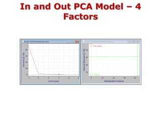
  • 35. In and Out PCA Model – 4 Factors
  • 36. Sample Residual in PCA • X = TPT + E • TPT describes the model. E is not the model, it is the residual variation that is not included in the model. In model – scores based. • A sample could have a large distance to the center of the model described by TPT, be far away from the center. Exceed the 95% confidence interval. Out model – residuals based. • A sample could also have a E larger than the 95% CI of the model. The sample residual exceeds the residual variation calculated with all the samples in the model. This is what happened to the 7.29% (w/w) sample + noise. Esbensen KH (2012) Multivariate Data Analysis- in practice. 5th edn. CAMO Software, and equation 5-23 in Pirouette manual.
  • 37. Sample Residual in PCA If a particular sample residual exceeds the residual of the model, it could be considered an outlier, “it might not belong to the same population as the other samples in the training set.” Pirouette manual, Sample Residual topic (5.23 – 5.28) An F-test is used (si is for the sample, s0 for the variance of model. A threshold is then calculated as shown in the plot
  • 38. Q-Statistic • This is referred to the squared prediction error. Q is related to the sample residual variance but without normalization. • Also used to evaluate whether a sample might be an outlier. The critical value of Q can be calculated from its approximate distribution. Pirouette manual, Chapter 5, Q-Statistic, equation 5.29
  • 39. Probability • Consider a probability cutoff of 95%. The null hypothesis is that the variances are equal. If the probability value corresponding to the F value exceeds 95% then the hypothesis is rejected, and it is inferred that the sample was not drawn from the same population. • As the samples probability approaches 1, then the chance that it is an outlier increases. Pirouette chapter 5, Probability (page 5-24)
  • 40. Mahalanobis Distance in PCA Pirouette manual, Chapter 5, page 5-25 Calculated for each sample, as a measure of variability. This is the distance from the multivariate mean. If a sample’s distance excees MDcrit, it may be an outlier.
  • 41. Understanding Hotelling’s T2 Test • In univariate statistics the t-test is used to estimate confidence interval for one variable. • This is the estimation of confidence interval for a multivariate system. • Confidence limits are built using the training set which would contain measurements that represent the normal (in control) situation. • The computed MD (the so-called T2 value) of each value is compared to a critical T2 value. • Used to build multivariate process control charts using the original variables or PCs.
  • 42. Principal Component Analysis (PCA)- Preamble to Quantitative Methods 42 Rodolfo J. Romañach, Ph.D. QUIM 6835 Chemometrcs February =------- 2022
  • 43. A.U. Vanarase, M. Alcalà, J.I. Jerez Rozo, F.J. Muzzio and R.J. Romañach, “Real-time monitoring of drug concentration in a continuous powder mixing process using NIR spectroscopy, Chemical Engineering Science, 2010, 65(21), 5728 – 5733. PCA Scores Plot-The Transition from Qualitative to Quantitative The first PC shows that concentration is the main source of variation in the data. This qualitative observation is a good positive indication that a good quantitative model can be developed.
  • 44. Introduction to Principal Component Analysis (PCA)- Discussion of Exercise 44 Rodolfo J. Romañach, Ph.D. QUIM 6835 Chemometrcs February =------- 2022
  • 45. Spectra and PCA Score Plot
  • 46. Spectra, PCA Score Plot, & Loadings Line Plot Comp No. M1.R2X M1.R2X(cum) Comp[1] 0.986703 0.986703 Comp[2] 0.0124451 0.999148 Orthogonality
  • 47. What is the objective? • If the goal is to determine differences in baseline, then method development is completed. • If the goal is to differentiate between samples of different concentrations then more work is needed. Pretreatment of the data becomes necessary.
  • 48. Spectra, PCA Score Plot, & Loadings Line Plot Comp No. M2.R2X M2.R2X Comp[1] 0.827293 0.827293 Comp[2] 0.146939 0.146939 Orthogonality
  • 49. PCA – Orthogonality Obtained for spectra of 0 -15% (w/w) without pretreatment. Notice that first factor summarizes most of the variation, and then it starts decreasing. Each factor summarizes new variation, not included in previous factors. Pretreatment was not used, only mean centering. PCA After only Mean-Centering Variance Percent Cumulative Press Cal Factor1 5.48197 98.67 98.67034 0.073874 Factor2 0.06914 1.2445 99.91486 0.00473 Factor3 0.00403 0.0726 99.98741 0.000699 Factor4 0.00032 0.0057 99.99308 0.000384 Factor5 0.00027 0.0049 99.99799 0.000111 Factor6 5.8E-05 0.001 99.99904 0.000053 Factor7 3.5E-05 0.0006 99.99967 0.000018 Factor8 8E-06 0.0002 99.99983 0.000009
  • 50.  If the spectral noise is known to be 0.1%, then how many principal components should be used to explain the data ?  Here we have the opportunity to filter or reduce the spectral noise since we do not have to keep the eight factors. Principal Components Analysis (PCA)
  • 51. 95% Confidence Interval The distance from the multivariate mean, commonly referred to as the Mahalanobis distance (MD), is computed with the scores. In Hotelling’s T2 test, the squared MD values are called Hotelling’s T2 values which are compared with a table of critical values. De Maesschalck, R.; Jouan-Rimbaud, D.; Massart, D. L., The Mahalanobis distance. Chemometrics Intellig. Lab. Syst. 2000, 50 (1), 1-18.
  • 52. Euclidean & Mahalonobis Distance The Euclidean distance would tell us the distance traveled. However, if there is bad weather or there are many airplanes trying to land the distance traveled would be greater. The distance traveled would not be the same for every flight. In that case we could calculate a Mahalanobis distance based on the standard deviations of the actual travel distances. The Mahalanobis distance is thus a statistical distance.
  • 53. Principal Component Analysis (PCA) Introduction to Outlier Diagnostics & Projections 53 Rodolfo J. Romañach, Ph.D. QUIM 6835 Chemometrcs September 3, 2019 Class no. 7
  • 54. Foods Example 2018 1. Spectra have been uploaded and category variables were added. 2. View the spectra. 3. Look at all spectra. Look at all flour spectra. 4. Perform 2nd derivative with 7 points. 5. Perform second derivative spectra. Savitzky Golay 19 points. 6. Select just one spectrum to view spectral differences. 7. Select limited number of spectra. 8. Look at all Flour spectra. Obtain shortened spectral range eliminating some of high frequency region. 9. Perform PCA of flour with 2nd der 19 points, in shortened spectral region (194-1063 variables).
  • 55. Foods Example 2018- 2 1. View scores plot, and Hotelling’s limits, loadings plot (line and score plot), influence plot, explained variance. 2. Examine sample no. 2 more closely. 3. Review In and Out for Flour model. 4. Residual vs. Hotelling. 5. Predict samples 6 -10 of flour, as if they were unknowns. These should be projected within 95% confidence interval. 6. Perform a PCA of the pan criollo samples. 7. Project Whole wheat into pan criollo.
  • 56. Vector Multiplication 56 For the product of two matrices to be defined, the number of columns of the first matrix must equal the number of rows of the second matrix. Show scores and loadings in software.
  • 57. Vector Multiplication  inner product, dot product, or scalar product, and seeing the vector as a one column or one row matrix.  The length of a vector is  Inner product obtained with vectors that have the same dimensions: x = [200 300 100 360] y = [380 580 420 840] x∙y = 200∙380 + 300∙580 + 100∙420 + 360∙840 x∙y = 594400 57 Matrix multiplication requires that the number of columns of first matrix = number of rows of second. m x n n x p = m x p Chapter 9 Vectors and matrices. In Data Handling in Science and Technology, Massart, D. L.; Vandeginste, B. G. M.; Buydens, L. M. C.; De Jong, S.; Lewi, P. J.; Smeyers-Verbeke, J., Eds. Elsevier: 1998; Vol. 20, pp 231-261.
  • 58. Vector Multiplication  Second way of writing the product, explains why it is called the dot product Matrix multiplication requires that the number of columns of first matrix = number of rows of second. m x n n x p = m x p Matrix multiplication is done by summing the products of ith element of a row with the ith element of a column. 58 Chapter 9 Vectors and matrices. In Data Handling in Science and Technology, Massart, D. L.; Vandeginste, B. G. M.; Buydens, L. M. C.; De Jong, S.; Lewi, P. J.; Smeyers-Verbeke, J., Eds. Elsevier: 1998; Vol. 20, pp 231-261.