


[PRML 3.1~3.2] Linear Regression / Bias-Variance Decomposition
- 1. © 2016. SNU CSE Biointelligence Lab., http://bi.snu.ac.kr Bayesian Linear Regression - part 1 1 곽동현 서울대학교 바이오지능 연구실
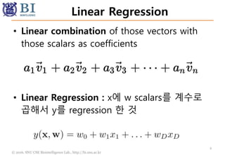
- 2. © 2016. SNU CSE Biointelligence Lab., http://bi.snu.ac.kr Linear Regression • Linear combination of those vectors with those scalars as coefficients 2 • Linear Regression : x에 w scalars를 계수로 곱해서 y를 regression 한 것
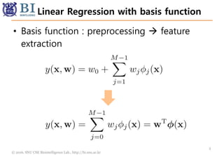
- 3. © 2016. SNU CSE Biointelligence Lab., http://bi.snu.ac.kr Linear Regression with basis function • Basis function : preprocessing feature extraction 3
- 4. © 2016. SNU CSE Biointelligence Lab., http://bi.snu.ac.kr Non-linear Regression • If the basis functions are non-linear, then the model is non-linear w.r.t input x. • Also the model is linear w.r.t feature(x). 4
- 5. © 2016. SNU CSE Biointelligence Lab., http://bi.snu.ac.kr Basis functions • Polynomial basis function • RBF(Radial basis function) (The normalization coefficient is unimportant because these basis functions will be multiplied by adaptive parameters wj.) 5
- 6. © 2016. SNU CSE Biointelligence Lab., http://bi.snu.ac.kr Basis functions • Sigmoidal basis function 6 a general linear combination of logistic sigmoid functions is equivalent to a general linear combination of ‘tanh’ functions.
- 7. © 2016. SNU CSE Biointelligence Lab., http://bi.snu.ac.kr Basis functions 7
- 8. © 2016. SNU CSE Biointelligence Lab., http://bi.snu.ac.kr Probabilistic Approach 8
- 9. © 2016. SNU CSE Biointelligence Lab., http://bi.snu.ac.kr MLE == Least Square • Why we use Least Square Loss? • Because of Maximum Likelihood Solution MLE를 위해 먼저 확률적인 접근을 도입 9
- 10. © 2016. SNU CSE Biointelligence Lab., http://bi.snu.ac.kr Mean is Mean 10
- 11. © 2016. SNU CSE Biointelligence Lab., http://bi.snu.ac.kr Likelihood • Vector formulation Likelihood (Identically independently distributed) 11
- 12. © 2016. SNU CSE Biointelligence Lab., http://bi.snu.ac.kr What is Likelihood? • X = {x1, x2, x3, … , xN} • T = {t1, t2, t3, … , tN} • Supervised Learning : X는 항상 conditioning p( T | Θ ; X ) • Unsupervised Learning p( X | Θ ) 12 ; 뒤에 오는 변수는 R.V가 아니고 deterministic vector 즉, 고정된 상수로 취급하는 것을 의미함
- 13. © 2016. SNU CSE Biointelligence Lab., http://bi.snu.ac.kr Supervised Learning • Supervised Learning X가 항상 conditioning variable에 위치함 ex) p( t | x ) • Unsupervised Learning X의 분포에 대해서도 관심이 있음 ex) p( x | x’ ) 13
- 14. © 2016. SNU CSE Biointelligence Lab., http://bi.snu.ac.kr In Supervised Learning • 우리는 Supervised learning을 할 것임. 따라서 x에 대한 conditioning은 notation에서 생략하기로 함 14
- 15. © 2016. SNU CSE Biointelligence Lab., http://bi.snu.ac.kr Log Likelihood 15
- 16. © 2016. SNU CSE Biointelligence Lab., http://bi.snu.ac.kr Maximum Loglikelihood LSE • Maximum Log Likelihood Gradient = 0 16 Least Square Error (Gradient = 0으로 놓고 풀 수 있는 이유는 Least Square Error가 quadratic form 이기 때문에 극한을 구하면 그 점이 항상 maximum 이라서 이다.)
- 17. © 2016. SNU CSE Biointelligence Lab., http://bi.snu.ac.kr Maximum Loglikelihood LSE • Maximum Log Likelihood Gradient = 0 17 • W에 대해서 정리한 다음, Vector notation사용
- 18. © 2016. SNU CSE Biointelligence Lab., http://bi.snu.ac.kr Maximum Loglikelihood LSE 18
- 19. © 2016. SNU CSE Biointelligence Lab., http://bi.snu.ac.kr Pseudo Inverse • 더 이상의 자세한 설명은 생략. • 다크프로그래머의 4. 특이값 분해(SVD)와 pseudo inverse, 최소자승법(least square method) 글을 참조하기 바람. http://darkpgmr.tistory.com/106 19
- 20. © 2016. SNU CSE Biointelligence Lab., http://bi.snu.ac.kr Stochastic Gradient Descent • Linear Regression의 Closed-form solution은 데이터의 N이 매우 큰데 컴퓨터의 cpu가 아주 안좋은 경우 느릴 수 있다. • 이런 경우 Gradient = 0 이 아니라, gradient descent 방법을 취할 수 있는데, 이 때에도 데 이터가 너무 많으면 stochastic gradient descent를 사용하면 효율적이다. 20
- 21. © 2016. SNU CSE Biointelligence Lab., http://bi.snu.ac.kr Geometry of least squares 21
- 22. © 2016. SNU CSE Biointelligence Lab., http://bi.snu.ac.kr Quadratic Regularization 22
- 23. © 2016. SNU CSE Biointelligence Lab., http://bi.snu.ac.kr Generalized Regularization • q =2 corresponds to the quadratic regularization. 23 q=4 이면 w는 sparsity의 반대되는 방향으로, w1과 w2값이 모두 0이 아닌 조건을 갖게 된다.
- 24. © 2016. SNU CSE Biointelligence Lab., http://bi.snu.ac.kr Sparse Weight 24 • Prior Regularization Lagrange Multiplier(해석) 실제로는 regularization term의 람 다는 고정된 크기의 boundary를 정하는 게 아니고, 마치 고무줄 처 럼 람다가 크면 더 경계가 줄어들 고, 람다가 0이되면 무한한 공간으 로 고무줄이 팽창하는 것이다. 그 러나 이해를 위해서 우선은 그냥 고정된 크기의 boundary를 갖는 constraint로 해석
- 25. © 2016. SNU CSE Biointelligence Lab., http://bi.snu.ac.kr Bias-Variance Decomposition 25
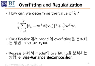
- 26. © 2016. SNU CSE Biointelligence Lab., http://bi.snu.ac.kr Overfitting and Regularization 26 • How can we determine the value of λ ? • Classification에서 model의 overfitting을 분석하 는 방법 VC anlaysis • Regression에서 model의 overfitting을 분석하는 방법 Bias-Variance decomposition
- 27. © 2016. SNU CSE Biointelligence Lab., http://bi.snu.ac.kr Bias and Variance 27
- 28. © 2016. SNU CSE Biointelligence Lab., http://bi.snu.ac.kr Out-of-sample Error • y(x) = y(x; w) : 즉, 우리가 학습시키는 모델 • h(x) : true underlying function (이세상의 존재하는 모든 데이터에 대한 평균) 28 • 이제부터는 다소 추상적인 개념이 등장함. Underlying true function / Model uncertainty
- 29. © 2016. SNU CSE Biointelligence Lab., http://bi.snu.ac.kr Out-of-sample Error • 즉 다음 수식의 의미는 true underlying function 과 우리가 학습한 모델의 squared loss임. 즉 test data에 대한 오차라고 해석 가능 (엄밀하게는 out-of-sample error임) 29
- 30. © 2016. SNU CSE Biointelligence Lab., http://bi.snu.ac.kr Uncertainty of model • Uncertainty of model은 다음과 같은 방법으로 분석함. 30 • 이것의 의미는 유한한 크기 데이터셋 D가 N개 만큼 존재할 때, 각 데이터셋에 대한 out-of-sample error를 평균 낸 것 • 즉 모델과 underlying function은 동일한데, 데이터셋을 샘 플링하면서 발생하는 노이즈를 해석하고자 함. • 그래서 이제 데이터셋 D에대한 평균 out-of-sample error 로 부터 model의 uncertainty를 유도할 것임
- 31. © 2016. SNU CSE Biointelligence Lab., http://bi.snu.ac.kr Bias-Variance Decomposition 31 수식을 전개한 다음 다시 정리 을 뺏다가 더해주고,에서
- 32. © 2016. SNU CSE Biointelligence Lab., http://bi.snu.ac.kr Bias-Variance Decomposition 32 여기에 D에 대한 평균을 취하면, 마지막 항(2ab)은 사라지게 된다. (그 이유는 a에 해당하는 term에서 E_D를 취하면 a=0이 되기 때문) = 0
- 33. © 2016. SNU CSE Biointelligence Lab., http://bi.snu.ac.kr Bias-Variance Decomposition • The first term, called the squared bias, represents the extent to which the average prediction over all data sets differs from the desired regression function. • The second term, called the variance, measures the extent to which the solutions for individual data sets vary around their average, 33 • Bias term : 임의의 D데이터로 학습한 모델 y(x;D)의 test error를 D에 대해 평균낸 것 모델이 데이터 포인트 를 모두 맞추면 0이 됨. • Variance term : 임의의 D데이터로 학습한 모델 y(x;D)과 그 모델들의 D에대한 평균E_D{y(x;D)}과의 편차^2의 평균을 구한 것. 즉 y(x;D)-mean(y(x;D)) 즉 편차가 큰 차이를 보인다면, 그 모델은 데이터셋에 따라서 크게 요 동을 치는 instable한 모델이 된다.(overfitting)
- 34. © 2016. SNU CSE Biointelligence Lab., http://bi.snu.ac.kr Bias-Variance • Bias : Specification accuracy of learning model 즉 데이터 D에서 발생한 y와 y_target의 차이. Training error로 해석 가능 • Variance : Generalization instability of learning model 이것은 동일한 분포에서 발생된 데이터셋 D1과 D2 를 학습시켰을 때, 두 모델 y(x,w)의 variance가 얼마 나 큰 가를 의미함. model의 instability 34
- 35. © 2016. SNU CSE Biointelligence Lab., http://bi.snu.ac.kr Bias-Variance Tradeoff • as we increase model complexity bias decreases (i.e., a better fit to data) variance increases (i.e., fit varies more with data) • Bias가 크다 model이 데이터를 제대로 예측하 지 못한다 underfitting • Variance가 크다 model이 데이터에 따라서 심하게 모양이 바뀐다 overfitting 35
- 36. © 2016. SNU CSE Biointelligence Lab., http://bi.snu.ac.kr Bias-Variance Tradeoff 36
- 37. © 2016. SNU CSE Biointelligence Lab., http://bi.snu.ac.kr Monte-Carlo Estimation • 실제로 여러 개의 데이터셋으로부터 bias와 variance 값을 측정해볼 수 있 다. 이를 통해 model complexity를 조절하거나 regularization 계수를 조정 할 수 있다. 37
- 38. © 2016. SNU CSE Biointelligence Lab., http://bi.snu.ac.kr THANK YOU 38