SlideShare a Scribd company logo
Data Mining Project
By Gabriele Angeletti
angeletti.gabriele@gmail.com
Image Similarity & Semi-Supervised Learning
Document Similarity:
Shingling + Locality Sensitive Hashing
Jaccard Distance = #(D1 ⋂ D2) / #(D1 ⋃ D2)
What about Image Similarity?
● Very high dimensional spaces
● Single dimension carries very little information
● Many variants and transformations (translation, rotation, scaling, lighting etc*)
● Computationally demanding
● Jaccard Distance performs poorly in this context
Locality Sensitive Hashing
Main idea: hash points in buckets, such that the nearer two points are, the more
likely they are to be hashed in the same bucket.
Need a definition of “near”, and a function that maps “nearby” points to the same
buckets.
LSH Family H: set of function H that is (d1, d2, p1, p2)-sensitive. For points q,p:
If D(p,q) < d1 then P(h(p) == h(q)) > p1
If D(p,q) > d2 then P(h(p) == h(q)) < p2
H: hash functions, D: definition of “near” (“far” actually).
LSH problems: many hyper-parameters to fine-tune, computationally expensive
LSH Forest
LSH index place each point p into a bucket with label g(p) = (h1(p), h2(p), . . . , hk(p)), g(p) is the k-digit label
assigned to point p.
LSH Forest, instead of assigning fixed-length labels to points, let the labels be of variable length; each label
is made long enough to ensure that every point has a distinct label. A maximum label length km is imposed.
The variable length label generation: let h1, h2, . . . , hkm be a sequence of km hash functions drawn
independently and uniformly at random from H. The length-x label of a point p is given by g(p, x) = (h1(p), h2
(p), . . . , hx(p)).
Ref: M. Bawa, T. Condie and P. Ganesan, “LSH Forest: Self-Tuning Indexes for Similarity Search”, WWW ‘05 Proceedings of the 14th
international conference on World Wide Web, 651-660, 2005.
LSH Forest (cont.)
LSH Tree: logical prefix tree on the set of all labels, with each leaf corresponding to a point.
LSH Forest: composed of L such LSH Trees, each constructed with an independently drawn random
sequence of hash functions from H.
Query processing (m nearest neighbors of point p):
Traversing the LSH Trees in two phases.
In the first top-down phase, find the leaf having the largest
prefix match with p’s label. x := maxl i{xi} is the bottom-most
level of leaf nodes across all L trees.
In the second bottom-up phase, we collect M points from
the LSH Forest, moving up from level x towards the root.
The M points are then ranked in order of decreasing
similarity with p and returned.
LSH Forest - test setting
Distance function: cosine distance
LSHForest implementation: sklearn
Hyper-parameters: default values of sklearn
Accuracy metric for the k-th nearest neighbor: (p / data_len)
p = 0
for each element in test set:
If label(element) == label(k nearest neighbor of element)
p++
This accuracy metric measures the ability of LSH Forest to retrieve elements of the same class.
LSH Forest - MNIST results
Dataset: MNIST - handwritten digits grayscale image dataset. 28x28 pixels per image
Training set - 50k images
Test set - 10k images
Dataset random samples:
LSH Forest accuracy@k for k = 1, … , 50 neighbors
Accuracy of ~95% for the first neighbor, drops to
~57% for the 50th neighbor.
LSH Forest - notMNIST results
Dataset: notMNIST - grayscale images of letters from A to J in different fonts. 28x28 pixels per image
Training set - 200k images
Test set - 10k images
Dataset random samples:
LSH Forest accuracy@k for k = 1, … , 50 neighbors
Accuracy of ~92% for the first neighbor, drops to
~70% for the 50th neighbor.
Can we do
better?
Idea: extract higher-level
features with semantic meaning.
How: Unsupervised Neural
Networks (Autoencoders)
● LSH Forest took 784 feature
vectors as input, treating each
pixel like a feature
● Extracting higher-level features
would:
- compress the data
- be computationally efficient
(features << 784)
- improve performance
(comparisons done between
features with semantic meaning
rather than raw pixels)
Autoencoders
Idea: Map input space to another space, and then
reconstruct the original input from that space.
The hope is that if the autoencoder is able to
reconstruct the original input from a lower dimensional
representation of if, it means that the representation
has successfully captured important features in the
input distribution.
The mappings are linear in the model parameters (W, b),
followed by a non-linearity, e.s. tanh(Wx + b).
The loss function is usually the l2 loss (mean squared error)
or the cross-entropy loss.
Autoencoders - math
Input x with dimension (N x P)
Model parameters:
- matrix W of dimension (P x H)
- vector bh of dimension H
- vector bv of dimension P
h = sigma(Wx + bh) // latent representation (encoder)
z = sigma(W’h + bv) // reconstruction (decoder)
loss = loss_function(x, z)
The parameters update rule is derived using backpropagation (i.e. computing
the gradients with respect to the chosen loss function).
theta’ = theta + learning_rate * gradient_wrt_theta
sigma() is a non-linear activation function (common choices are sigmoid and tanh)
Denoising Autoencoders
Autoencoder variant trained to reconstruct the original input starting from a
corrupted version of it (denoising task).
Idea: If the autoencoder is able to reconstruct the input ( )
from a corrupted version of it ( ) we can expect that it must have
captured robust features in the latent representation.
Corruption method used - masking noise: a random fraction v of pixels
is set to 0. Other possible methods: salt-and-pepper noise (fraction v
flipped to minimum or maximum value), gaussian noise.
x~ = noise(x)
h = sigma(Wx~ + bh) // latent representation (encoder)
z = sigma(W’h + bv) // reconstruction (decoder)
loss = loss_function(x, z)
Stacked (Denoising) Autoencoders
We can take the latent representation learned by an autoencoder, and use it as
training data for a second autoencoder. In this way, we can create
a stack of autoencoders, where each layer learns a higher-level
representation of the input distribution with respect to the layer
below it. It can be theoretically proved that adding a layer to the stack
will improve the variational bound on the log probability of the data,
if the layers are trained properly.
This procedure is called unsupervised pre-training.
Once the autoencoders are trained, we can construct the final architecture
(deep autoencoder) and perform unsupervised fine-tuning of all the
layers together.
Deep Autoencoder - visualize high-level features
Visualization: t-distributed stochastic neighbor embedding (t-SNE)
Left: t-SNE of the original MNIST (784 to 2), Right: t-SNE of the latent representation of a trained deep autoencoder (64 to 2)
Combine Deep
Autoencoders
with LSH Forest
● Deep Autoencoders extract high-level
meaningful features (encodings)
● Encodings dimension is typically much
lower than original dimension (data
compression + computational efficiency)
● Similarity can be computed at the
encodings level rather than pixel level (i.
e. similarity between two high-level
features (e.g. eyes) is much more
meaningful than similarity between pairs
of pixels
● This more powerful similarity detection
algorithm can be used in semi-
supervised settings (more on that later)
Deep Autoencoder + LSH Forest - MNIST
- Deep Autoencoder architecture:
4 encoders - 784 → 2048 → 1024 → 256 → 64
4 decoders - 64 → 256 → 1024 → 2048 → 784
- LSH Forest ran on 64d encodings
- Sample reconstructions of the model:
LSH Forest accuracy@k for k = 1, … , 50 neighbors
Similar accuracy for the first neighbors, +~35%
deep autoencoder improvement for 50th neighbor
Deep Autoencoder + LSH Forest - notMNIST
- Deep Autoencoder architecture:
4 encoders - 784 → 2048 → 1024 → 256 → 64
4 decoders - 64 → 256 → 1024 → 2048 → 784
- LSH Forest ran on 64d encodings
- Sample reconstructions of the model:
LSH Forest accuracy@k for k = 1, … , 50 neighbors
Similar accuracy for the first neighbors, +~16%
deep autoencoder improvement for 50th neighbor
Deep Autoencoder + LSH Forest - Query results
MNIST: query image: , neighbors indexes: 1, 6, 12, 20, 27, 36, 50
Basic LSH (n. of 2: 17/50) Deep Autoencoder + LSH (n. of 2: 50/50)
notMNIST: query image: , neighbors indexes: 1, 6, 12, 20, 27, 36, 50
Basic LSH (n. Of G: 7/50) Deep Autoencoder + LSH (n. Of G: 37/50)
Can we exploit
better similarity
techniques in
semi-supervised
settings?
● Big Data (unlabeled data >>>> labeled data)
● Supervised learning algorithms need labels
● Assumption: dataset with k% unlabeled data
(say 98%) and j% labeled data (say 2%)
● Can we infer the labels of the 98% of the
data using the labels we have for the 2%?
● Deep Autoencoder + LSH is totally
unsupervised: we can use 100% of the data
● Idea: estimate the label of an item with the
label of the most similar item for which we
have the label
Two approaches
First Found: Assign the label of the
most similar item for which the label
is known.
Majority Voting: Assign the most
frequent label between neighbors.
The two results are nearly identical between
the two approaches.
Result: By knowing only 2750 / 55000 (5%) of
the labels in the training set, we can infer the
labels for the test set with a ~95% accuracy.
Two more metrics
The average position of the first neighbor
with known label decreases as the number
of known labels increases. Thus, the more
labels we know, the less neighbors we have
to compute with LSH.
The average number of not found elements with
known label decreases as the number of known
label increases. For this not found elements, a
random label is chosen. Anyway, for just 5% of
known labels, avg not founds are just 0.2.
Future work:
● Try majority voting weighted on distances
● Try convolutional autoencoders instead of denoising
autoencoders (Huge expected improvement especially
with images, provides translation and rotation invariance)
● Try with more complex datasets (e.g. CIFAR-10, 32x32
color images)
● Try the approach with other domains (e.g. sound, text, ...)
● Object similarity between domains (e.g. image of two
similar to sound of person spelling “two”)

More Related Content

What's hot (19)

PPTX
Dijkstra's algorithm presentation
Subid Biswas
 
PPTX
Dstar Lite
Adrian Sotelo
 
PDF
Encoding survey
Rajeev Raman
 
PPTX
Ch03 Mining Massive Data Sets stanford
Sakthivel C R
 
PDF
Density Based Clustering
SSA KPI
 
PDF
The Power of Motif Counting Theory, Algorithms, and Applications for Large Gr...
Nesreen K. Ahmed
 
PPTX
DBSCAN : A Clustering Algorithm
Pınar Yahşi
 
PPT
5.4 randomized datastructures
Krish_ver2
 
PDF
Linear sorting
Krishna Chaytaniah
 
PDF
High-Performance Graph Analysis and Modeling
Nesreen K. Ahmed
 
PDF
IJCAI13 Paper review: Large-scale spectral clustering on graphs
Akisato Kimura
 
PDF
Sortsearch
Krishna Chaytaniah
 
PDF
Chromatic Sparse Learning
Databricks
 
PDF
DASH: A C++ PGAS Library for Distributed Data Structures and Parallel Algorit...
Menlo Systems GmbH
 
PPT
Uninformed search
Bablu Shofi
 
PPTX
Dbscan algorithom
Mahbubur Rahman Shimul
 
Dijkstra's algorithm presentation
Subid Biswas
 
Dstar Lite
Adrian Sotelo
 
Encoding survey
Rajeev Raman
 
Ch03 Mining Massive Data Sets stanford
Sakthivel C R
 
Density Based Clustering
SSA KPI
 
The Power of Motif Counting Theory, Algorithms, and Applications for Large Gr...
Nesreen K. Ahmed
 
DBSCAN : A Clustering Algorithm
Pınar Yahşi
 
5.4 randomized datastructures
Krish_ver2
 
Linear sorting
Krishna Chaytaniah
 
High-Performance Graph Analysis and Modeling
Nesreen K. Ahmed
 
IJCAI13 Paper review: Large-scale spectral clustering on graphs
Akisato Kimura
 
Chromatic Sparse Learning
Databricks
 
DASH: A C++ PGAS Library for Distributed Data Structures and Parallel Algorit...
Menlo Systems GmbH
 
Uninformed search
Bablu Shofi
 
Dbscan algorithom
Mahbubur Rahman Shimul
 

Viewers also liked (11)

PDF
Multidimensional Data in the VO
Jose Enrique Ruiz
 
PPTX
Agile Testing - LAST Conference 2015
Theresa Neate
 
PDF
A survey on massively Parallelism for indexing multidimensional datasets on t...
Tejovat Technologies Pvt.Ltd.,Wakad
 
PPT
Multidimensional Indexing
Digvijay Singh
 
PDF
Multidimensional Analysis of Complex Networks
Lino Possamai
 
PPTX
pratik meshram-Unit 5 (contemporary mkt r sch)
Pratik Meshram
 
PPTX
K-means Clustering with Scikit-Learn
Sarah Guido
 
PDF
Locality Sensitive Hashing By Spark
Spark Summit
 
PDF
차원축소 훑어보기 (PCA, SVD, NMF)
beom kyun choi
 
PPTX
Visualization using tSNE
Yan Xu
 
PPT
12. Indexing and Hashing in DBMS
koolkampus
 
Multidimensional Data in the VO
Jose Enrique Ruiz
 
Agile Testing - LAST Conference 2015
Theresa Neate
 
A survey on massively Parallelism for indexing multidimensional datasets on t...
Tejovat Technologies Pvt.Ltd.,Wakad
 
Multidimensional Indexing
Digvijay Singh
 
Multidimensional Analysis of Complex Networks
Lino Possamai
 
pratik meshram-Unit 5 (contemporary mkt r sch)
Pratik Meshram
 
K-means Clustering with Scikit-Learn
Sarah Guido
 
Locality Sensitive Hashing By Spark
Spark Summit
 
차원축소 훑어보기 (PCA, SVD, NMF)
beom kyun choi
 
Visualization using tSNE
Yan Xu
 
12. Indexing and Hashing in DBMS
koolkampus
 
Ad

Similar to Project - Deep Locality Sensitive Hashing (20)

PPTX
Clique and sting
Subramanyam Natarajan
 
PPTX
Deep learning from mashine learning AI..
premkumarlive
 
PDF
Similarity Search in High Dimensions via Hashing
Maruf Aytekin
 
PDF
Machine Learning Algorithms Introduction.pdf
Vinodh58
 
PDF
Computer Vision: Feature matching with RANSAC Algorithm
allyn joy calcaben
 
PDF
ENBIS 2018 presentation on Deep k-Means
tthonet
 
PPTX
Deep Learning for Search
Bhaskar Mitra
 
PPTX
Deep Learning for Search
Bhaskar Mitra
 
PPTX
Introduction to Deep Learning and Tensorflow
Oswald Campesato
 
PPT
MapReduceAlgorithms.ppt
CheeWeiTan10
 
PDF
MS CS - Selecting Machine Learning Algorithm
Kaniska Mandal
 
PPTX
Anomaly detection using deep one class classifier
홍배 김
 
PPTX
Deep Learning and Watson Studio
Sasha Lazarevic
 
PPTX
Deep Learning: R with Keras and TensorFlow
Oswald Campesato
 
PDF
Building graphs to discover information by David Martínez at Big Data Spain 2015
Big Data Spain
 
PDF
Enterprise Scale Topological Data Analysis Using Spark
Spark Summit
 
PDF
Enterprise Scale Topological Data Analysis Using Spark
Alpine Data
 
PDF
[241]large scale search with polysemous codes
NAVER D2
 
PDF
Query Optimization - Brandon Latronica
"FENG "GEORGE"" YU
 
PPTX
feature matching and model fitting .pptx
demepa1337
 
Clique and sting
Subramanyam Natarajan
 
Deep learning from mashine learning AI..
premkumarlive
 
Similarity Search in High Dimensions via Hashing
Maruf Aytekin
 
Machine Learning Algorithms Introduction.pdf
Vinodh58
 
Computer Vision: Feature matching with RANSAC Algorithm
allyn joy calcaben
 
ENBIS 2018 presentation on Deep k-Means
tthonet
 
Deep Learning for Search
Bhaskar Mitra
 
Deep Learning for Search
Bhaskar Mitra
 
Introduction to Deep Learning and Tensorflow
Oswald Campesato
 
MapReduceAlgorithms.ppt
CheeWeiTan10
 
MS CS - Selecting Machine Learning Algorithm
Kaniska Mandal
 
Anomaly detection using deep one class classifier
홍배 김
 
Deep Learning and Watson Studio
Sasha Lazarevic
 
Deep Learning: R with Keras and TensorFlow
Oswald Campesato
 
Building graphs to discover information by David Martínez at Big Data Spain 2015
Big Data Spain
 
Enterprise Scale Topological Data Analysis Using Spark
Spark Summit
 
Enterprise Scale Topological Data Analysis Using Spark
Alpine Data
 
[241]large scale search with polysemous codes
NAVER D2
 
Query Optimization - Brandon Latronica
"FENG "GEORGE"" YU
 
feature matching and model fitting .pptx
demepa1337
 
Ad

Recently uploaded (20)

PPTX
Q1_Science 8_Week3-Day 1.pptx science lesson
AizaRazonado
 
PDF
A Man of the Forest: The Contributions of Gifford Pinchot
RowanSales
 
PDF
Calcium in a supernova remnant as a fingerprint of a sub-Chandrasekhar-mass e...
Sérgio Sacani
 
PDF
A High-Caliber View of the Bullet Cluster through JWST Strong and Weak Lensin...
Sérgio Sacani
 
PDF
The ALMA-CRISTAL survey: Gas, dust, and stars in star-forming galaxies when t...
Sérgio Sacani
 
PPTX
770043401-q1-Ppt-pe-and-Health-7-week-1-lesson-1.pptx
AizaRazonado
 
PDF
Carbonate formation and fluctuating habitability on Mars
Sérgio Sacani
 
PDF
Unit-3 ppt.pdf organic chemistry - 3 unit 3
visionshukla007
 
PDF
oil and gas chemical injection system
Okeke Livinus
 
PPTX
ION EXCHANGE CHROMATOGRAPHY NEW PPT (JA).pptx
adhagalejotshna
 
PDF
Pharmakon of algorithmic alchemy: Marketing in the age of AI
Selcen Ozturkcan
 
DOCX
Critical Book Review (CBR) - "Hate Speech: Linguistic Perspectives"
Sahmiral Amri Rajagukguk
 
PPTX
Diagnostic Features of Common Oral Ulcerative Lesions.pptx
Dr Palak borade
 
PDF
Preserving brand authenticity amid AI-driven misinformation: Sustaining consu...
Selcen Ozturkcan
 
PDF
Global Congress on Forensic Science and Research
infoforensicscience2
 
PDF
Plankton and Fisheries Bovas Joel Notes.pdf
J. Bovas Joel BFSc
 
PPTX
Q1 - W1 - D2 - Models of matter for science.pptx
RyanCudal3
 
PPTX
Bacillus thuringiensis.crops & golden rice
priyadharshini87125
 
PDF
The emergence of galactic thin and thick discs across cosmic history
Sérgio Sacani
 
PPT
Restriction digestion of DNA for students of undergraduate and post graduate ...
DrMukeshRameshPimpli
 
Q1_Science 8_Week3-Day 1.pptx science lesson
AizaRazonado
 
A Man of the Forest: The Contributions of Gifford Pinchot
RowanSales
 
Calcium in a supernova remnant as a fingerprint of a sub-Chandrasekhar-mass e...
Sérgio Sacani
 
A High-Caliber View of the Bullet Cluster through JWST Strong and Weak Lensin...
Sérgio Sacani
 
The ALMA-CRISTAL survey: Gas, dust, and stars in star-forming galaxies when t...
Sérgio Sacani
 
770043401-q1-Ppt-pe-and-Health-7-week-1-lesson-1.pptx
AizaRazonado
 
Carbonate formation and fluctuating habitability on Mars
Sérgio Sacani
 
Unit-3 ppt.pdf organic chemistry - 3 unit 3
visionshukla007
 
oil and gas chemical injection system
Okeke Livinus
 
ION EXCHANGE CHROMATOGRAPHY NEW PPT (JA).pptx
adhagalejotshna
 
Pharmakon of algorithmic alchemy: Marketing in the age of AI
Selcen Ozturkcan
 
Critical Book Review (CBR) - "Hate Speech: Linguistic Perspectives"
Sahmiral Amri Rajagukguk
 
Diagnostic Features of Common Oral Ulcerative Lesions.pptx
Dr Palak borade
 
Preserving brand authenticity amid AI-driven misinformation: Sustaining consu...
Selcen Ozturkcan
 
Global Congress on Forensic Science and Research
infoforensicscience2
 
Plankton and Fisheries Bovas Joel Notes.pdf
J. Bovas Joel BFSc
 
Q1 - W1 - D2 - Models of matter for science.pptx
RyanCudal3
 
Bacillus thuringiensis.crops & golden rice
priyadharshini87125
 
The emergence of galactic thin and thick discs across cosmic history
Sérgio Sacani
 
Restriction digestion of DNA for students of undergraduate and post graduate ...
DrMukeshRameshPimpli
 

Project - Deep Locality Sensitive Hashing

  • 2. Image Similarity & Semi-Supervised Learning Document Similarity: Shingling + Locality Sensitive Hashing Jaccard Distance = #(D1 ⋂ D2) / #(D1 ⋃ D2) What about Image Similarity? ● Very high dimensional spaces ● Single dimension carries very little information ● Many variants and transformations (translation, rotation, scaling, lighting etc*) ● Computationally demanding ● Jaccard Distance performs poorly in this context
  • 3. Locality Sensitive Hashing Main idea: hash points in buckets, such that the nearer two points are, the more likely they are to be hashed in the same bucket. Need a definition of “near”, and a function that maps “nearby” points to the same buckets. LSH Family H: set of function H that is (d1, d2, p1, p2)-sensitive. For points q,p: If D(p,q) < d1 then P(h(p) == h(q)) > p1 If D(p,q) > d2 then P(h(p) == h(q)) < p2 H: hash functions, D: definition of “near” (“far” actually). LSH problems: many hyper-parameters to fine-tune, computationally expensive
  • 4. LSH Forest LSH index place each point p into a bucket with label g(p) = (h1(p), h2(p), . . . , hk(p)), g(p) is the k-digit label assigned to point p. LSH Forest, instead of assigning fixed-length labels to points, let the labels be of variable length; each label is made long enough to ensure that every point has a distinct label. A maximum label length km is imposed. The variable length label generation: let h1, h2, . . . , hkm be a sequence of km hash functions drawn independently and uniformly at random from H. The length-x label of a point p is given by g(p, x) = (h1(p), h2 (p), . . . , hx(p)). Ref: M. Bawa, T. Condie and P. Ganesan, “LSH Forest: Self-Tuning Indexes for Similarity Search”, WWW ‘05 Proceedings of the 14th international conference on World Wide Web, 651-660, 2005.
  • 5. LSH Forest (cont.) LSH Tree: logical prefix tree on the set of all labels, with each leaf corresponding to a point. LSH Forest: composed of L such LSH Trees, each constructed with an independently drawn random sequence of hash functions from H. Query processing (m nearest neighbors of point p): Traversing the LSH Trees in two phases. In the first top-down phase, find the leaf having the largest prefix match with p’s label. x := maxl i{xi} is the bottom-most level of leaf nodes across all L trees. In the second bottom-up phase, we collect M points from the LSH Forest, moving up from level x towards the root. The M points are then ranked in order of decreasing similarity with p and returned.
  • 6. LSH Forest - test setting Distance function: cosine distance LSHForest implementation: sklearn Hyper-parameters: default values of sklearn Accuracy metric for the k-th nearest neighbor: (p / data_len) p = 0 for each element in test set: If label(element) == label(k nearest neighbor of element) p++ This accuracy metric measures the ability of LSH Forest to retrieve elements of the same class.
  • 7. LSH Forest - MNIST results Dataset: MNIST - handwritten digits grayscale image dataset. 28x28 pixels per image Training set - 50k images Test set - 10k images Dataset random samples: LSH Forest accuracy@k for k = 1, … , 50 neighbors Accuracy of ~95% for the first neighbor, drops to ~57% for the 50th neighbor.
  • 8. LSH Forest - notMNIST results Dataset: notMNIST - grayscale images of letters from A to J in different fonts. 28x28 pixels per image Training set - 200k images Test set - 10k images Dataset random samples: LSH Forest accuracy@k for k = 1, … , 50 neighbors Accuracy of ~92% for the first neighbor, drops to ~70% for the 50th neighbor.
  • 9. Can we do better? Idea: extract higher-level features with semantic meaning. How: Unsupervised Neural Networks (Autoencoders) ● LSH Forest took 784 feature vectors as input, treating each pixel like a feature ● Extracting higher-level features would: - compress the data - be computationally efficient (features << 784) - improve performance (comparisons done between features with semantic meaning rather than raw pixels)
  • 10. Autoencoders Idea: Map input space to another space, and then reconstruct the original input from that space. The hope is that if the autoencoder is able to reconstruct the original input from a lower dimensional representation of if, it means that the representation has successfully captured important features in the input distribution. The mappings are linear in the model parameters (W, b), followed by a non-linearity, e.s. tanh(Wx + b). The loss function is usually the l2 loss (mean squared error) or the cross-entropy loss.
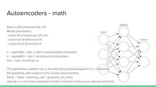
  • 11. Autoencoders - math Input x with dimension (N x P) Model parameters: - matrix W of dimension (P x H) - vector bh of dimension H - vector bv of dimension P h = sigma(Wx + bh) // latent representation (encoder) z = sigma(W’h + bv) // reconstruction (decoder) loss = loss_function(x, z) The parameters update rule is derived using backpropagation (i.e. computing the gradients with respect to the chosen loss function). theta’ = theta + learning_rate * gradient_wrt_theta sigma() is a non-linear activation function (common choices are sigmoid and tanh)
  • 12. Denoising Autoencoders Autoencoder variant trained to reconstruct the original input starting from a corrupted version of it (denoising task). Idea: If the autoencoder is able to reconstruct the input ( ) from a corrupted version of it ( ) we can expect that it must have captured robust features in the latent representation. Corruption method used - masking noise: a random fraction v of pixels is set to 0. Other possible methods: salt-and-pepper noise (fraction v flipped to minimum or maximum value), gaussian noise. x~ = noise(x) h = sigma(Wx~ + bh) // latent representation (encoder) z = sigma(W’h + bv) // reconstruction (decoder) loss = loss_function(x, z)
  • 13. Stacked (Denoising) Autoencoders We can take the latent representation learned by an autoencoder, and use it as training data for a second autoencoder. In this way, we can create a stack of autoencoders, where each layer learns a higher-level representation of the input distribution with respect to the layer below it. It can be theoretically proved that adding a layer to the stack will improve the variational bound on the log probability of the data, if the layers are trained properly. This procedure is called unsupervised pre-training. Once the autoencoders are trained, we can construct the final architecture (deep autoencoder) and perform unsupervised fine-tuning of all the layers together.
  • 14. Deep Autoencoder - visualize high-level features Visualization: t-distributed stochastic neighbor embedding (t-SNE) Left: t-SNE of the original MNIST (784 to 2), Right: t-SNE of the latent representation of a trained deep autoencoder (64 to 2)
  • 15. Combine Deep Autoencoders with LSH Forest ● Deep Autoencoders extract high-level meaningful features (encodings) ● Encodings dimension is typically much lower than original dimension (data compression + computational efficiency) ● Similarity can be computed at the encodings level rather than pixel level (i. e. similarity between two high-level features (e.g. eyes) is much more meaningful than similarity between pairs of pixels ● This more powerful similarity detection algorithm can be used in semi- supervised settings (more on that later)
  • 16. Deep Autoencoder + LSH Forest - MNIST - Deep Autoencoder architecture: 4 encoders - 784 → 2048 → 1024 → 256 → 64 4 decoders - 64 → 256 → 1024 → 2048 → 784 - LSH Forest ran on 64d encodings - Sample reconstructions of the model: LSH Forest accuracy@k for k = 1, … , 50 neighbors Similar accuracy for the first neighbors, +~35% deep autoencoder improvement for 50th neighbor
  • 17. Deep Autoencoder + LSH Forest - notMNIST - Deep Autoencoder architecture: 4 encoders - 784 → 2048 → 1024 → 256 → 64 4 decoders - 64 → 256 → 1024 → 2048 → 784 - LSH Forest ran on 64d encodings - Sample reconstructions of the model: LSH Forest accuracy@k for k = 1, … , 50 neighbors Similar accuracy for the first neighbors, +~16% deep autoencoder improvement for 50th neighbor
  • 18. Deep Autoencoder + LSH Forest - Query results MNIST: query image: , neighbors indexes: 1, 6, 12, 20, 27, 36, 50 Basic LSH (n. of 2: 17/50) Deep Autoencoder + LSH (n. of 2: 50/50) notMNIST: query image: , neighbors indexes: 1, 6, 12, 20, 27, 36, 50 Basic LSH (n. Of G: 7/50) Deep Autoencoder + LSH (n. Of G: 37/50)
  • 19. Can we exploit better similarity techniques in semi-supervised settings? ● Big Data (unlabeled data >>>> labeled data) ● Supervised learning algorithms need labels ● Assumption: dataset with k% unlabeled data (say 98%) and j% labeled data (say 2%) ● Can we infer the labels of the 98% of the data using the labels we have for the 2%? ● Deep Autoencoder + LSH is totally unsupervised: we can use 100% of the data ● Idea: estimate the label of an item with the label of the most similar item for which we have the label
  • 20. Two approaches First Found: Assign the label of the most similar item for which the label is known. Majority Voting: Assign the most frequent label between neighbors. The two results are nearly identical between the two approaches. Result: By knowing only 2750 / 55000 (5%) of the labels in the training set, we can infer the labels for the test set with a ~95% accuracy.
  • 21. Two more metrics The average position of the first neighbor with known label decreases as the number of known labels increases. Thus, the more labels we know, the less neighbors we have to compute with LSH. The average number of not found elements with known label decreases as the number of known label increases. For this not found elements, a random label is chosen. Anyway, for just 5% of known labels, avg not founds are just 0.2.
  • 22. Future work: ● Try majority voting weighted on distances ● Try convolutional autoencoders instead of denoising autoencoders (Huge expected improvement especially with images, provides translation and rotation invariance) ● Try with more complex datasets (e.g. CIFAR-10, 32x32 color images) ● Try the approach with other domains (e.g. sound, text, ...) ● Object similarity between domains (e.g. image of two similar to sound of person spelling “two”)