SlideShare a Scribd company logo
Discontinuous Hamiltonian Monte Carlo
for discontinuous and discrete distributions
Aki Nishimura
joint work with David Dunson and Jianfeng Lu
SAMSI Workshop: Trends and Advances in Monte Carlo Sampling Algorithms
December 12, 2017
Models with discrete params / discontinuous likelihoods
Discrete : unknown population size, change points
Discontinuous : nonparametric generalized Bayes, threshold effects
Hamiltonian Monte Carlo (HMC) for Bayesian computation
Bayesian inference often relies on Markov chain Monte Carlo.
HMC has become popular as an efficient general-purpose algorithm:
allows for more flexible generative models (e.g. non-conjugacy).
a critical building block of probabilistic programming languages.
Hamiltonian Monte Carlo (HMC) for Bayesian computation
Idea of a probabilistic programming language: you specify the model,
then the software takes care of the rest.
Hamiltonian Monte Carlo (HMC) for Bayesian computation
Idea of a probabilistic programming language: you specify the model,
then the software takes care of the rest.
Probabilistic programming languages can algorithmically evaluate
(unnormalized) log posterior density.
(unnormalized) log conditional densities efficiently by taking
advantage of conditional independence structure.
gradients of log density.
HMC is well-suited to such softwares and has demonstrated
a number of empirical successes e.g. through Stan and PyMC.
better theoretical scalability in the number of parameters
(Beskos et al., 2013).
HMC and discrete parameters / discontinuous likelihoods
HMC is based on solutions of an ordinary differential equation.
But the ODE makes no sense for discrete parameters / discontinuous
likelihoods.
HMC and discrete parameters / discontinuous likelihoods
HMC is based on solutions of an ordinary differential equation.
But the ODE makes no sense for discrete parameters / discontinuous
likelihoods.
HMC’s inability to handle discrete parameters is considered the most
serious drawback (Gelman et al., 2015; Monnahan et al., 2016).
Existing approaches in special cases:
smooth surrogate function for binary pairwise Markov random
field models (Zhang et al., 2012).
treat discrete parameters as continuous if the likelihood still
makes sense (Berger et al., 2012).
Our approach: discontinous HMC
Features:
allows for a discontinuous target distribution.
handles discrete parameters through embedding them into a
continuous space.
fits within the framework of probabilistic programming languages.
Our approach: discontinous HMC
Features:
allows for a discontinuous target distribution.
handles discrete parameters through embedding them into a
continuous space.
fits within the framework of probabilistic programming languages.
Techniques:
is motivated by theory of measure-valued differential equation &
event-driven Monte Carlo.
is based on a novel numerical method for discontinuous dynamics.
Theoretical properties:
generalizes (and hence outperforms) variable-at-a-time Metropolis.
achieves a high acceptance rate that indicates a scaling property
comparable to HMC.
Review of HMC
Table of Contents
1 Review of HMC
2 Turning discrete problems into discontinuous ones
3 Theory of discontinuous Hamiltonian dynamics
4 Numerical method for discontinuous dynamics
5 Numerical results
6 Results
Review of HMC
HMC in its basic form
HMC samples from an augmented parameter space (θ, p) where:
π(θ, p) ∝ πΘ(θ) × N (p ; 0, mI)
U(θ) = − log πΘ(θ) is called potential energy.
Review of HMC
HMC in its basic form
HMC samples from an augmented parameter space (θ, p) where:
π(θ, p) ∝ πΘ(θ) × N (p ; 0, mI)
U(θ) = − log πΘ(θ) is called potential energy.
Transition rule of HMC
Given the current state (θ0, p0), HMC generates the next state as follows:
1 Re-sample p0 ∼ N (0, mI)
2 Generate a Metropolis proposal by solving Hamilton’s equation:
dθ
dt
= m−1
p,
dp
dt
= − θU(θ) (1)
with the initial condition (θ0, p0).
3 Accept or reject the proposal.
Interpretation of (1): dθ
dt = velocity, mass × d
dt (velocity) = − θU(θ)
Review of HMC
Visual illustration: HMC in action
HMC for a 2d Gaussian (correlation = 0.9)
Review of HMC
HMC in a more general form
HMC samples from an augmented parameter space (θ, p) where:
π(θ, p) ∝ πΘ(θ) × πP (p)
K(p) = − log πP (p) is called kinetic energy.
Transition rule of HMC
Given the current state (θ0, p0), HMC generates the next state as follows:
1 Re-sample p0 ∼ πP (·).
2 Generate a Metropolis proposal by solving Hamilton’s equation:
dθ
dt
= pK(p)
dp
dt
= − θU(θ) (2)
with the initial condition (θ0, p0).
3 Accept or reject the proposal.
Review of HMC
Properties of Hamiltonian dynamics
Conservation of energy:
U(θ(t)) + K(p(t)) = U(θ0) + K(p0) for all t ∈ R
a basis for high acceptance probabilities of HMC proposals.
Review of HMC
Properties of Hamiltonian dynamics
Conservation of energy:
U(θ(t)) + K(p(t)) = U(θ0) + K(p0) for all t ∈ R
a basis for high acceptance probabilities of HMC proposals.
Reversibility & Volume-preservation
symmetry of proposals “P(x → x∗) = P(x∗ → x)”
Turning discrete problems into discontinuous ones
Table of Contents
1 Review of HMC
2 Turning discrete problems into discontinuous ones
3 Theory of discontinuous Hamiltonian dynamics
4 Numerical method for discontinuous dynamics
5 Numerical results
6 Results
Turning discrete problems into discontinuous ones
Turning discrete problem into discontinuous one
Consider a discrete parameter N ∈ Z+ with a prior πN (·).
Map N into a continuous parameter N such that
N = n if and only if N ∈ (an, an+1]
To match the distribution of N, the corresponding density of N is
πN
(˜n) =
n≥1
πN (n)
an+1 − an
1{an < ˜n ≤ an+1}
Turning discrete problems into discontinuous ones
Turning discrete problem into discontinuous one
0 2 4 6 8 10
n
0.0
0.2
0.4
0.6
Massfunction
pmf (n+1) 2
0 2 4 6 8 10
n
0.0
0.2
0.4
0.6
Density
log-scale
embedding
linear-scale
embedding
Figure: Relating a discrete mass function (left) to a density function (right).
Turning discrete problems into discontinuous ones
What about more complex discrete spaces?
Graphs? Trees?
For “momentum” to be useful, we need a notion of direction.
Turning discrete problems into discontinuous ones
What about more complex discrete spaces?
Short answer: I don’t know. (Let me know if you got ideas.)
Graphs? Trees?
For “momentum” to be useful, we need a notion of direction.
Theory of discontinuous Hamiltonian dynamics
Table of Contents
1 Review of HMC
2 Turning discrete problems into discontinuous ones
3 Theory of discontinuous Hamiltonian dynamics
4 Numerical method for discontinuous dynamics
5 Numerical results
6 Results
Theory of discontinuous Hamiltonian dynamics
When U(θ) = − log π(θ) is discontinuous, Hamilton’s equations
dθ
dt
= pK(p)
dp
dt
= − θU(θ) (3)
becomes a measure-valued differential equation / inclusion.
θi
U(θ)
Figure:
Theory of discontinuous Hamiltonian dynamics
Define discontinuous dynamics as a limit of smooth dynamics:
Uδ — smooth approximations of U i.e. limδ→0 Uδ = U.
(θδ, pδ)(t) — the solution corresponding to Uδ.
θi
U(θ)
Uδ(θ)
Figure:
Theory of discontinuous Hamiltonian dynamics
Define discontinuous dynamics as a limit of smooth dynamics:
Uδ — smooth approximations of U i.e. limδ→0 Uδ = U.
(θδ, pδ)(t) — the solution corresponding to Uδ.
(θ, p)(t) := limδ→0(θδ, pδ)(t).
θi
U(θ)
Uδ(θ)
Figure: Example trajectory θ(t) of discontinuous Hamiltonian dynamics.
Theory of discontinuous Hamiltonian dynamics
Behavior of dynamics at discontinuity
When the trajectory θ(t) encounters a discontinuity of U at event
time te, the momentum p(t) undergoes an instantaneous change.
Theory of discontinuous Hamiltonian dynamics
Behavior of dynamics at discontinuity
When the trajectory θ(t) encounters a discontinuity of U at event
time te, the momentum p(t) undergoes an instantaneous change.
The change in p occurs only in the direction of “− θU(θ)”:
p(t+
e ) = p(t−
e ) − γ ν (θ(te))
where ν(θ) is orthonormal to the discontinuity boundary of U.
The scalar γ is determined by the energy conservation principle:
K(p(t+
e )) − K(p(t−
e )) = U(θ(t−
e )) − U(θ(t+
e ))
(provided K(p) is convex and K(p) → ∞ as p → ∞).
Numerical method for discontinuous dynamics
Table of Contents
1 Review of HMC
2 Turning discrete problems into discontinuous ones
3 Theory of discontinuous Hamiltonian dynamics
4 Numerical method for discontinuous dynamics
5 Numerical results
6 Results
Numerical method for discontinuous dynamics
Dealing with discontinuity
Numerical method for discontinuous dynamics
Dealing with discontinuity
How about ignoring them?
Numerical method for discontinuous dynamics
Dealing with discontinuity
How about ignoring them?
Leapfrog integrator completely fails to preserve the energy.
i.e. low (or even negligible) acceptance probabilities.
Numerical method for discontinuous dynamics
Event-driven approach at discontinuity
Pakman and Paninski (2013) and Afshar and Domke (2015):
Detect discontinuities and treat them appropriately.
(Event-driven Monte Carlo of Alder and Wainwright (1959).)
Numerical method for discontinuous dynamics
Event-driven approach at discontinuity
Pakman and Paninski (2013) and Afshar and Domke (2015):
Detect discontinuities and treat them appropriately.
(Event-driven Monte Carlo of Alder and Wainwright (1959).)
Problem: in Gaussian momentum case, the change in U(θ) must be
computed across every single discontinuity.
Numerical method for discontinuous dynamics
Problem with Gaussian momentum & existing approach
Say var(N) ≈ 1, 000. Then a Metropolis step N → N ± 1, 000
should have a good chance of acceptance.
The numerical method requires 1, 000 density evaluations (ouch!)
for a corresponding transition.
ΔU ≈ .01
Figure: Conditional distribution of an embedded discrete parameter in
the Jolly-Seber example.
Numerical method for discontinuous dynamics
Laplace momentum: better alternative
Consider a Laplace momentum π(p) ∝ i exp(−m−1
i |pi|).
The corresponding Hamilton’s equation is
dθ
dt
= m−1
· sign(p),
dp
dt
= − θU(θ)
Numerical method for discontinuous dynamics
Laplace momentum: better alternative
Consider a Laplace momentum π(p) ∝ i exp(−m−1
i |pi|).
The corresponding Hamilton’s equation is
dθ
dt
= m−1
· sign(p),
dp
dt
= − θU(θ)
Key property: the velocity dθ/dt depends only on the signs of pi’s
and not on their magnitudes.
This property allows an accurate numerical approximation
without keeping track of small changes in pi’s.
Numerical method for discontinuous dynamics
Numerical method for Laplace momentum
Observation: approximating dynamics based on Laplace momentum is
simple in a 1-D case — dθ/dt = m−1 sign(p), dp/dt = − U(θ)
θ θ* = θ + Δt × m-1 sign(p)
U(θ)
p
Numerical method for discontinuous dynamics
Numerical method for Laplace momentum
Observation: approximating dynamics based on Laplace momentum is
simple in a 1-D case — dθ/dt = m−1 sign(p), dp/dt = − U(θ)
θ θ* = θ + Δt × m-1 sign(p)
U(θ)
p U(θ*) − U(θ) < K(p) ?
Numerical method for discontinuous dynamics
Numerical method for Laplace momentum
Observation: approximating dynamics based on Laplace momentum is
simple in a 1-D case — dθ/dt = m−1 sign(p), dp/dt = − U(θ)
θ θ* = θ + Δt × m-1 sign(p)
U(θ)
U(θ*) − U(θ) = K(p) − K(p*)
p*
Numerical method for discontinuous dynamics
Numerical method for Laplace momentum
Observation: approximating dynamics based on Laplace momentum is
simple in a 1-D case — dθ/dt = m−1 sign(p), dp/dt = − U(θ)
θ θ*
U(θ*) − U(θ)
p
Numerical method for discontinuous dynamics
Numerical method for Laplace momentum
Observation: approximating dynamics based on Laplace momentum is
simple in a 1-D case — dθ/dt = m−1 sign(p), dp/dt = − U(θ)
p* ← - p
θ* ← θ
Numerical method for discontinuous dynamics
Coordinate-wise integration for Laplace momentum
For θ ∈ Rd, we can split the ODE into its coordinate-wise component:
dθi
dt
= m−1
i sign(pi),
dpi
dt
= −∂θi
U(θ),
dθ−i
dt
=
dp−i
dt
= 0 (4)
Numerical method for discontinuous dynamics
Coordinate-wise integration for Laplace momentum
4 2 0 2
4
2
0
2
4
0
1
2
3
4
5
Figure: Trajectory of a numerical solution via the coordinate-wise integrator.
Numerical method for discontinuous dynamics
Coordinate-wise integration for Laplace momentum
Reversibility preserved by symmetric splitting or randomly permuting
the coordinates.
We can also use Laplace momentum for discrete parameters and
Gaussian momentum for continuous parameters.
Numerical method for discontinuous dynamics
Properties of discontinuous HMC
When using independent Laplace momentum,
Proposals are rejection-free thanks to exact energy conservation.1
1
But too big of a stepsize leads to poor mixing.
Numerical method for discontinuous dynamics
Properties of discontinuous HMC
When using independent Laplace momentum,
Proposals are rejection-free thanks to exact energy conservation.1
Taking one numerical integration step of DHMC
≡
Variable-at-a-time Metropolis.
When mixing Laplace and Gaussian momentum:
Errors in energy is O(∆t2), and hence 1 − O(∆t4) acceptance rate.
1
But too big of a stepsize leads to poor mixing.
Numerical results
Table of Contents
1 Review of HMC
2 Turning discrete problems into discontinuous ones
3 Theory of discontinuous Hamiltonian dynamics
4 Numerical method for discontinuous dynamics
5 Numerical results
6 Results
Numerical results
Numerical results: Jolly-Seber (capture-recapture) model
Data : the number of marked / unmarked individuals over multiple
capture occasions
Parameters : population sizes, capture probabilities, survival rates
Numerical results
Numerical results: Jolly-Seber model
One computational challenge arises from unidentifiability between an
unknown capture probability qi and population size Ni.
0 5
log(q1/(1 q1))
2.0
2.5
3.0
log10(N1)
Numerical results
Numerical results: Jolly-Seber model
Table: Performance summary of each algorithm on the Jolly-Serber example.
ESS per 100 samples ESS per minute Path length Iter time
DHMC (diagonal) 45.5 424 45 87.7
DHMC (identity) 24.1 126 77.5 157
NUTS-Gibbs 1.04 6.38 150 133
Metropolis 0.0714 58.5 1 1
ESS : effective sample sizes (minimum over
the first and second moment estimators)
diagonal / identity : choice of mass matrix
Metropolis : optimal random walk Metropolis
NUTS-Gibbs : alternate update of continuous &
discrete params as employed by PyMC
Numerical results
Numerical results: generalized Bayesian inference
For a given loss function (y, θ) of interest, a generalized posterior
(Bissiri et al., 2016) is given by
πpost(θ) ∝ exp − i (yi, θ) πprior(θ)
We consider a binary classification with the 0-1 loss
(y, θ) = 1{y = sign(x θ)} for y ∈ {−1, 1}.
9.2 9.0 8.8
Intercept
0
2
4
6
Density(conditional)
Numerical results
Numerical results: generalized Bayesian inference
Data: semiconductor quality with various sensor measurements
Goal: predict faulty products / infer relevant sensor measurements
Numerical results
Numerical results: generalized Bayesian inference
Table: Performance summary on the generalized Bayesian posterior example.
ESS per 100 samples ESS per minute Path length Iter time
DHMC 26.3 76 25 972
Metropolis 0.00809 (± 0.0018) 0.227 1 1
Variable-at-a-time 0.514 (± 0.039) 39.8 1 36.2
9.2 9.0 8.8
Intercept
0
2
4
6
Density(conditional)
Results
Table of Contents
1 Review of HMC
2 Turning discrete problems into discontinuous ones
3 Theory of discontinuous Hamiltonian dynamics
4 Numerical method for discontinuous dynamics
5 Numerical results
6 Results
Results
Summary
Hamiltonian dynamics based on Laplace momentum allows an
efficient exploration of discontinuous target distributions.
Numerical method with exact energy conservation property.
Results
Future directions
Test DHMC on a wider range of applications in the context of a
probabilistic programming language.
Explore the utility of Laplace momentum as an alternative to
Gaussian one.
What to do with more complex discrete spaces?
Develop notion of directions.
Avoid rejections by “swapping” probability between θ and p.
Results
References
Nishimura, A., Dunson, D. and Lu, J. (2017) “Discontinuous Hamiltonian
Monte Carlo for sampling discrete parameters,” arXiv:1705.08510.
Code available at
https://github.com/aki-nishimura/discontinuous-hmc
Results
The End
Thank you!

More Related Content

PDF
QMC Program: Trends and Advances in Monte Carlo Sampling Algorithms Workshop,...
The Statistical and Applied Mathematical Sciences Institute
 
PDF
QMC Program: Trends and Advances in Monte Carlo Sampling Algorithms Workshop,...
The Statistical and Applied Mathematical Sciences Institute
 
PDF
QMC Program: Trends and Advances in Monte Carlo Sampling Algorithms Workshop,...
The Statistical and Applied Mathematical Sciences Institute
 
PDF
QMC Program: Trends and Advances in Monte Carlo Sampling Algorithms Workshop,...
The Statistical and Applied Mathematical Sciences Institute
 
PDF
QMC Program: Trends and Advances in Monte Carlo Sampling Algorithms Workshop,...
The Statistical and Applied Mathematical Sciences Institute
 
PDF
QMC Program: Trends and Advances in Monte Carlo Sampling Algorithms Workshop,...
The Statistical and Applied Mathematical Sciences Institute
 
PDF
QMC Program: Trends and Advances in Monte Carlo Sampling Algorithms Workshop,...
The Statistical and Applied Mathematical Sciences Institute
 
PDF
Unbiased Bayes for Big Data
Christian Robert
 
QMC Program: Trends and Advances in Monte Carlo Sampling Algorithms Workshop,...
The Statistical and Applied Mathematical Sciences Institute
 
QMC Program: Trends and Advances in Monte Carlo Sampling Algorithms Workshop,...
The Statistical and Applied Mathematical Sciences Institute
 
QMC Program: Trends and Advances in Monte Carlo Sampling Algorithms Workshop,...
The Statistical and Applied Mathematical Sciences Institute
 
QMC Program: Trends and Advances in Monte Carlo Sampling Algorithms Workshop,...
The Statistical and Applied Mathematical Sciences Institute
 
QMC Program: Trends and Advances in Monte Carlo Sampling Algorithms Workshop,...
The Statistical and Applied Mathematical Sciences Institute
 
QMC Program: Trends and Advances in Monte Carlo Sampling Algorithms Workshop,...
The Statistical and Applied Mathematical Sciences Institute
 
QMC Program: Trends and Advances in Monte Carlo Sampling Algorithms Workshop,...
The Statistical and Applied Mathematical Sciences Institute
 
Unbiased Bayes for Big Data
Christian Robert
 

What's hot (20)

PDF
MCMC and likelihood-free methods
Christian Robert
 
PDF
QMC Program: Trends and Advances in Monte Carlo Sampling Algorithms Workshop,...
The Statistical and Applied Mathematical Sciences Institute
 
PDF
Maximum likelihood estimation of regularisation parameters in inverse problem...
Valentin De Bortoli
 
PDF
Program on Quasi-Monte Carlo and High-Dimensional Sampling Methods for Applie...
The Statistical and Applied Mathematical Sciences Institute
 
PDF
Bayesian hybrid variable selection under generalized linear models
Caleb (Shiqiang) Jin
 
PDF
Delayed acceptance for Metropolis-Hastings algorithms
Christian Robert
 
PDF
Approximate Bayesian Computation with Quasi-Likelihoods
Stefano Cabras
 
PDF
Richard Everitt's slides
Christian Robert
 
PDF
QMC Opening Workshop, High Accuracy Algorithms for Interpolating and Integrat...
The Statistical and Applied Mathematical Sciences Institute
 
PDF
Chris Sherlock's slides
Christian Robert
 
PDF
Program on Quasi-Monte Carlo and High-Dimensional Sampling Methods for Applie...
The Statistical and Applied Mathematical Sciences Institute
 
PDF
Mark Girolami's Read Paper 2010
Christian Robert
 
PDF
Jere Koskela slides
Christian Robert
 
PDF
Rao-Blackwellisation schemes for accelerating Metropolis-Hastings algorithms
Christian Robert
 
PDF
Program on Quasi-Monte Carlo and High-Dimensional Sampling Methods for Applie...
The Statistical and Applied Mathematical Sciences Institute
 
PDF
ABC in Venezia
Christian Robert
 
PDF
Can we estimate a constant?
Christian Robert
 
PDF
Program on Quasi-Monte Carlo and High-Dimensional Sampling Methods for Applie...
The Statistical and Applied Mathematical Sciences Institute
 
PDF
Nested sampling
Christian Robert
 
PDF
Coordinate sampler: A non-reversible Gibbs-like sampler
Christian Robert
 
MCMC and likelihood-free methods
Christian Robert
 
QMC Program: Trends and Advances in Monte Carlo Sampling Algorithms Workshop,...
The Statistical and Applied Mathematical Sciences Institute
 
Maximum likelihood estimation of regularisation parameters in inverse problem...
Valentin De Bortoli
 
Program on Quasi-Monte Carlo and High-Dimensional Sampling Methods for Applie...
The Statistical and Applied Mathematical Sciences Institute
 
Bayesian hybrid variable selection under generalized linear models
Caleb (Shiqiang) Jin
 
Delayed acceptance for Metropolis-Hastings algorithms
Christian Robert
 
Approximate Bayesian Computation with Quasi-Likelihoods
Stefano Cabras
 
Richard Everitt's slides
Christian Robert
 
QMC Opening Workshop, High Accuracy Algorithms for Interpolating and Integrat...
The Statistical and Applied Mathematical Sciences Institute
 
Chris Sherlock's slides
Christian Robert
 
Program on Quasi-Monte Carlo and High-Dimensional Sampling Methods for Applie...
The Statistical and Applied Mathematical Sciences Institute
 
Mark Girolami's Read Paper 2010
Christian Robert
 
Jere Koskela slides
Christian Robert
 
Rao-Blackwellisation schemes for accelerating Metropolis-Hastings algorithms
Christian Robert
 
Program on Quasi-Monte Carlo and High-Dimensional Sampling Methods for Applie...
The Statistical and Applied Mathematical Sciences Institute
 
ABC in Venezia
Christian Robert
 
Can we estimate a constant?
Christian Robert
 
Program on Quasi-Monte Carlo and High-Dimensional Sampling Methods for Applie...
The Statistical and Applied Mathematical Sciences Institute
 
Nested sampling
Christian Robert
 
Coordinate sampler: A non-reversible Gibbs-like sampler
Christian Robert
 
Ad

Similar to QMC Program: Trends and Advances in Monte Carlo Sampling Algorithms Workshop, Discontinuous Hamiltonian Monte Carlo for Sampling Discrete Parameters - Aki Nishimura, Dec 12, 2017 (20)

PPTX
Introduction to hmc
Kota Takeda
 
PDF
Talk at 2013 WSC, ISI Conference in Hong Kong, August 26, 2013
Christian Robert
 
PDF
The slides of my Ph.D. defense
Apostolos Chalkis
 
PDF
HMC and NUTS
Marco Banterle
 
PDF
Deep Learning for Cyber Security
Altoros
 
PPTX
Monte Carlo Berkeley.pptx
HaibinSu2
 
PDF
Metropolis-Hastings MCMC Short Tutorial
Ralph Schlosser
 
PDF
intro
ssuser9ed16a1
 
ODP
Implementation of Variational Inference for Non-Parametric Hidden Markov Models
James McInerney
 
PPTX
Bayesian Neural Networks
Natan Katz
 
PPTX
planning and decision making
AdengappaUnavu
 
PDF
Unbiased Markov chain Monte Carlo methods
Pierre Jacob
 
PPTX
Hamiltonian Circuit
SauravGupta129
 
PPTX
Hamiltonian cycle in data structure 2
Home
 
PDF
Firefly exact MCMC for Big Data
Gianvito Siciliano
 
PDF
Markov chain monte_carlo_methods_for_machine_learning
Andres Mendez-Vazquez
 
PDF
How to Accelerate Molecular Simulations with Data? by Žofia Trsťanová, Machin...
Paris Women in Machine Learning and Data Science
 
PDF
2018 MUMS Fall Course - Bayesian inference for model calibration in UQ - Ralp...
The Statistical and Applied Mathematical Sciences Institute
 
ODP
Monte Carlo Methods
James Bell
 
PDF
An overview of Hidden Markov Models (HMM)
ananth
 
Introduction to hmc
Kota Takeda
 
Talk at 2013 WSC, ISI Conference in Hong Kong, August 26, 2013
Christian Robert
 
The slides of my Ph.D. defense
Apostolos Chalkis
 
HMC and NUTS
Marco Banterle
 
Deep Learning for Cyber Security
Altoros
 
Monte Carlo Berkeley.pptx
HaibinSu2
 
Metropolis-Hastings MCMC Short Tutorial
Ralph Schlosser
 
Implementation of Variational Inference for Non-Parametric Hidden Markov Models
James McInerney
 
Bayesian Neural Networks
Natan Katz
 
planning and decision making
AdengappaUnavu
 
Unbiased Markov chain Monte Carlo methods
Pierre Jacob
 
Hamiltonian Circuit
SauravGupta129
 
Hamiltonian cycle in data structure 2
Home
 
Firefly exact MCMC for Big Data
Gianvito Siciliano
 
Markov chain monte_carlo_methods_for_machine_learning
Andres Mendez-Vazquez
 
How to Accelerate Molecular Simulations with Data? by Žofia Trsťanová, Machin...
Paris Women in Machine Learning and Data Science
 
2018 MUMS Fall Course - Bayesian inference for model calibration in UQ - Ralp...
The Statistical and Applied Mathematical Sciences Institute
 
Monte Carlo Methods
James Bell
 
An overview of Hidden Markov Models (HMM)
ananth
 
Ad

More from The Statistical and Applied Mathematical Sciences Institute (20)

PDF
Causal Inference Opening Workshop - Latent Variable Models, Causal Inference,...
The Statistical and Applied Mathematical Sciences Institute
 
PDF
2019 Fall Series: Special Guest Lecture - 0-1 Phase Transitions in High Dimen...
The Statistical and Applied Mathematical Sciences Institute
 
PDF
Causal Inference Opening Workshop - Causal Discovery in Neuroimaging Data - F...
The Statistical and Applied Mathematical Sciences Institute
 
PDF
Causal Inference Opening Workshop - Smooth Extensions to BART for Heterogeneo...
The Statistical and Applied Mathematical Sciences Institute
 
PDF
Causal Inference Opening Workshop - A Bracketing Relationship between Differe...
The Statistical and Applied Mathematical Sciences Institute
 
PDF
Causal Inference Opening Workshop - Testing Weak Nulls in Matched Observation...
The Statistical and Applied Mathematical Sciences Institute
 
PPTX
Causal Inference Opening Workshop - Difference-in-differences: more than meet...
The Statistical and Applied Mathematical Sciences Institute
 
PDF
Causal Inference Opening Workshop - New Statistical Learning Methods for Esti...
The Statistical and Applied Mathematical Sciences Institute
 
PDF
Causal Inference Opening Workshop - Bipartite Causal Inference with Interfere...
The Statistical and Applied Mathematical Sciences Institute
 
PPTX
Causal Inference Opening Workshop - Bridging the Gap Between Causal Literatur...
The Statistical and Applied Mathematical Sciences Institute
 
PDF
Causal Inference Opening Workshop - Some Applications of Reinforcement Learni...
The Statistical and Applied Mathematical Sciences Institute
 
PDF
Causal Inference Opening Workshop - Bracketing Bounds for Differences-in-Diff...
The Statistical and Applied Mathematical Sciences Institute
 
PDF
Causal Inference Opening Workshop - Assisting the Impact of State Polcies: Br...
The Statistical and Applied Mathematical Sciences Institute
 
PDF
Causal Inference Opening Workshop - Experimenting in Equilibrium - Stefan Wag...
The Statistical and Applied Mathematical Sciences Institute
 
PDF
Causal Inference Opening Workshop - Targeted Learning for Causal Inference Ba...
The Statistical and Applied Mathematical Sciences Institute
 
PDF
Causal Inference Opening Workshop - Bayesian Nonparametric Models for Treatme...
The Statistical and Applied Mathematical Sciences Institute
 
PPTX
2019 Fall Series: Special Guest Lecture - Adversarial Risk Analysis of the Ge...
The Statistical and Applied Mathematical Sciences Institute
 
PPTX
2019 Fall Series: Professional Development, Writing Academic Papers…What Work...
The Statistical and Applied Mathematical Sciences Institute
 
PDF
2019 GDRR: Blockchain Data Analytics - Machine Learning in/for Blockchain: Fu...
The Statistical and Applied Mathematical Sciences Institute
 
PDF
2019 GDRR: Blockchain Data Analytics - QuTrack: Model Life Cycle Management f...
The Statistical and Applied Mathematical Sciences Institute
 
Causal Inference Opening Workshop - Latent Variable Models, Causal Inference,...
The Statistical and Applied Mathematical Sciences Institute
 
2019 Fall Series: Special Guest Lecture - 0-1 Phase Transitions in High Dimen...
The Statistical and Applied Mathematical Sciences Institute
 
Causal Inference Opening Workshop - Causal Discovery in Neuroimaging Data - F...
The Statistical and Applied Mathematical Sciences Institute
 
Causal Inference Opening Workshop - Smooth Extensions to BART for Heterogeneo...
The Statistical and Applied Mathematical Sciences Institute
 
Causal Inference Opening Workshop - A Bracketing Relationship between Differe...
The Statistical and Applied Mathematical Sciences Institute
 
Causal Inference Opening Workshop - Testing Weak Nulls in Matched Observation...
The Statistical and Applied Mathematical Sciences Institute
 
Causal Inference Opening Workshop - Difference-in-differences: more than meet...
The Statistical and Applied Mathematical Sciences Institute
 
Causal Inference Opening Workshop - New Statistical Learning Methods for Esti...
The Statistical and Applied Mathematical Sciences Institute
 
Causal Inference Opening Workshop - Bipartite Causal Inference with Interfere...
The Statistical and Applied Mathematical Sciences Institute
 
Causal Inference Opening Workshop - Bridging the Gap Between Causal Literatur...
The Statistical and Applied Mathematical Sciences Institute
 
Causal Inference Opening Workshop - Some Applications of Reinforcement Learni...
The Statistical and Applied Mathematical Sciences Institute
 
Causal Inference Opening Workshop - Bracketing Bounds for Differences-in-Diff...
The Statistical and Applied Mathematical Sciences Institute
 
Causal Inference Opening Workshop - Assisting the Impact of State Polcies: Br...
The Statistical and Applied Mathematical Sciences Institute
 
Causal Inference Opening Workshop - Experimenting in Equilibrium - Stefan Wag...
The Statistical and Applied Mathematical Sciences Institute
 
Causal Inference Opening Workshop - Targeted Learning for Causal Inference Ba...
The Statistical and Applied Mathematical Sciences Institute
 
Causal Inference Opening Workshop - Bayesian Nonparametric Models for Treatme...
The Statistical and Applied Mathematical Sciences Institute
 
2019 Fall Series: Special Guest Lecture - Adversarial Risk Analysis of the Ge...
The Statistical and Applied Mathematical Sciences Institute
 
2019 Fall Series: Professional Development, Writing Academic Papers…What Work...
The Statistical and Applied Mathematical Sciences Institute
 
2019 GDRR: Blockchain Data Analytics - Machine Learning in/for Blockchain: Fu...
The Statistical and Applied Mathematical Sciences Institute
 
2019 GDRR: Blockchain Data Analytics - QuTrack: Model Life Cycle Management f...
The Statistical and Applied Mathematical Sciences Institute
 

Recently uploaded (20)

PPTX
TEF & EA Bsc Nursing 5th sem.....BBBpptx
AneetaSharma15
 
PPTX
Care of patients with elImination deviation.pptx
AneetaSharma15
 
PDF
What is CFA?? Complete Guide to the Chartered Financial Analyst Program
sp4989653
 
DOCX
Action Plan_ARAL PROGRAM_ STAND ALONE SHS.docx
Levenmartlacuna1
 
PPTX
HEALTH CARE DELIVERY SYSTEM - UNIT 2 - GNM 3RD YEAR.pptx
Priyanshu Anand
 
PPTX
How to Track Skills & Contracts Using Odoo 18 Employee
Celine George
 
PPTX
Dakar Framework Education For All- 2000(Act)
santoshmohalik1
 
PPTX
Applications of matrices In Real Life_20250724_091307_0000.pptx
gehlotkrish03
 
PPTX
Cleaning Validation Ppt Pharmaceutical validation
Ms. Ashatai Patil
 
DOCX
SAROCES Action-Plan FOR ARAL PROGRAM IN DEPED
Levenmartlacuna1
 
PPTX
family health care settings home visit - unit 6 - chn 1 - gnm 1st year.pptx
Priyanshu Anand
 
PDF
2.Reshaping-Indias-Political-Map.ppt/pdf/8th class social science Exploring S...
Sandeep Swamy
 
PDF
Virat Kohli- the Pride of Indian cricket
kushpar147
 
PPTX
How to Apply for a Job From Odoo 18 Website
Celine George
 
PPTX
Five Point Someone – Chetan Bhagat | Book Summary & Analysis by Bhupesh Kushwaha
Bhupesh Kushwaha
 
PDF
Biological Classification Class 11th NCERT CBSE NEET.pdf
NehaRohtagi1
 
PPTX
Python-Application-in-Drug-Design by R D Jawarkar.pptx
Rahul Jawarkar
 
PPTX
20250924 Navigating the Future: How to tell the difference between an emergen...
McGuinness Institute
 
PPTX
A Smarter Way to Think About Choosing a College
Cyndy McDonald
 
PPTX
How to Close Subscription in Odoo 18 - Odoo Slides
Celine George
 
TEF & EA Bsc Nursing 5th sem.....BBBpptx
AneetaSharma15
 
Care of patients with elImination deviation.pptx
AneetaSharma15
 
What is CFA?? Complete Guide to the Chartered Financial Analyst Program
sp4989653
 
Action Plan_ARAL PROGRAM_ STAND ALONE SHS.docx
Levenmartlacuna1
 
HEALTH CARE DELIVERY SYSTEM - UNIT 2 - GNM 3RD YEAR.pptx
Priyanshu Anand
 
How to Track Skills & Contracts Using Odoo 18 Employee
Celine George
 
Dakar Framework Education For All- 2000(Act)
santoshmohalik1
 
Applications of matrices In Real Life_20250724_091307_0000.pptx
gehlotkrish03
 
Cleaning Validation Ppt Pharmaceutical validation
Ms. Ashatai Patil
 
SAROCES Action-Plan FOR ARAL PROGRAM IN DEPED
Levenmartlacuna1
 
family health care settings home visit - unit 6 - chn 1 - gnm 1st year.pptx
Priyanshu Anand
 
2.Reshaping-Indias-Political-Map.ppt/pdf/8th class social science Exploring S...
Sandeep Swamy
 
Virat Kohli- the Pride of Indian cricket
kushpar147
 
How to Apply for a Job From Odoo 18 Website
Celine George
 
Five Point Someone – Chetan Bhagat | Book Summary & Analysis by Bhupesh Kushwaha
Bhupesh Kushwaha
 
Biological Classification Class 11th NCERT CBSE NEET.pdf
NehaRohtagi1
 
Python-Application-in-Drug-Design by R D Jawarkar.pptx
Rahul Jawarkar
 
20250924 Navigating the Future: How to tell the difference between an emergen...
McGuinness Institute
 
A Smarter Way to Think About Choosing a College
Cyndy McDonald
 
How to Close Subscription in Odoo 18 - Odoo Slides
Celine George
 

QMC Program: Trends and Advances in Monte Carlo Sampling Algorithms Workshop, Discontinuous Hamiltonian Monte Carlo for Sampling Discrete Parameters - Aki Nishimura, Dec 12, 2017

  • 1. Discontinuous Hamiltonian Monte Carlo for discontinuous and discrete distributions Aki Nishimura joint work with David Dunson and Jianfeng Lu SAMSI Workshop: Trends and Advances in Monte Carlo Sampling Algorithms December 12, 2017
  • 2. Models with discrete params / discontinuous likelihoods Discrete : unknown population size, change points Discontinuous : nonparametric generalized Bayes, threshold effects
  • 3. Hamiltonian Monte Carlo (HMC) for Bayesian computation Bayesian inference often relies on Markov chain Monte Carlo. HMC has become popular as an efficient general-purpose algorithm: allows for more flexible generative models (e.g. non-conjugacy). a critical building block of probabilistic programming languages.
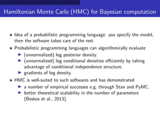
  • 4. Hamiltonian Monte Carlo (HMC) for Bayesian computation Idea of a probabilistic programming language: you specify the model, then the software takes care of the rest.
  • 5. Hamiltonian Monte Carlo (HMC) for Bayesian computation Idea of a probabilistic programming language: you specify the model, then the software takes care of the rest. Probabilistic programming languages can algorithmically evaluate (unnormalized) log posterior density. (unnormalized) log conditional densities efficiently by taking advantage of conditional independence structure. gradients of log density.
  • 6. Hamiltonian Monte Carlo (HMC) for Bayesian computation Idea of a probabilistic programming language: you specify the model, then the software takes care of the rest. Probabilistic programming languages can algorithmically evaluate (unnormalized) log posterior density. (unnormalized) log conditional densities efficiently by taking advantage of conditional independence structure. gradients of log density. HMC is well-suited to such softwares and has demonstrated a number of empirical successes e.g. through Stan and PyMC. better theoretical scalability in the number of parameters (Beskos et al., 2013).
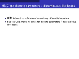
  • 7. HMC and discrete parameters / discontinuous likelihoods HMC is based on solutions of an ordinary differential equation. But the ODE makes no sense for discrete parameters / discontinuous likelihoods.
  • 8. HMC and discrete parameters / discontinuous likelihoods HMC is based on solutions of an ordinary differential equation. But the ODE makes no sense for discrete parameters / discontinuous likelihoods. HMC’s inability to handle discrete parameters is considered the most serious drawback (Gelman et al., 2015; Monnahan et al., 2016).
  • 9. HMC and discrete parameters / discontinuous likelihoods HMC is based on solutions of an ordinary differential equation. But the ODE makes no sense for discrete parameters / discontinuous likelihoods. HMC’s inability to handle discrete parameters is considered the most serious drawback (Gelman et al., 2015; Monnahan et al., 2016). Existing approaches in special cases: smooth surrogate function for binary pairwise Markov random field models (Zhang et al., 2012). treat discrete parameters as continuous if the likelihood still makes sense (Berger et al., 2012).
  • 10. Our approach: discontinous HMC Features: allows for a discontinuous target distribution. handles discrete parameters through embedding them into a continuous space. fits within the framework of probabilistic programming languages.
  • 11. Our approach: discontinous HMC Features: allows for a discontinuous target distribution. handles discrete parameters through embedding them into a continuous space. fits within the framework of probabilistic programming languages. Techniques: is motivated by theory of measure-valued differential equation & event-driven Monte Carlo. is based on a novel numerical method for discontinuous dynamics.
  • 12. Our approach: discontinous HMC Features: allows for a discontinuous target distribution. handles discrete parameters through embedding them into a continuous space. fits within the framework of probabilistic programming languages. Techniques: is motivated by theory of measure-valued differential equation & event-driven Monte Carlo. is based on a novel numerical method for discontinuous dynamics. Theoretical properties: generalizes (and hence outperforms) variable-at-a-time Metropolis. achieves a high acceptance rate that indicates a scaling property comparable to HMC.
  • 13. Review of HMC Table of Contents 1 Review of HMC 2 Turning discrete problems into discontinuous ones 3 Theory of discontinuous Hamiltonian dynamics 4 Numerical method for discontinuous dynamics 5 Numerical results 6 Results
  • 14. Review of HMC HMC in its basic form HMC samples from an augmented parameter space (θ, p) where: π(θ, p) ∝ πΘ(θ) × N (p ; 0, mI) U(θ) = − log πΘ(θ) is called potential energy.
  • 15. Review of HMC HMC in its basic form HMC samples from an augmented parameter space (θ, p) where: π(θ, p) ∝ πΘ(θ) × N (p ; 0, mI) U(θ) = − log πΘ(θ) is called potential energy. Transition rule of HMC Given the current state (θ0, p0), HMC generates the next state as follows: 1 Re-sample p0 ∼ N (0, mI) 2 Generate a Metropolis proposal by solving Hamilton’s equation: dθ dt = m−1 p, dp dt = − θU(θ) (1) with the initial condition (θ0, p0). 3 Accept or reject the proposal.
  • 16. Review of HMC HMC in its basic form HMC samples from an augmented parameter space (θ, p) where: π(θ, p) ∝ πΘ(θ) × N (p ; 0, mI) U(θ) = − log πΘ(θ) is called potential energy. Transition rule of HMC Given the current state (θ0, p0), HMC generates the next state as follows: 1 Re-sample p0 ∼ N (0, mI) 2 Generate a Metropolis proposal by solving Hamilton’s equation: dθ dt = m−1 p, dp dt = − θU(θ) (1) with the initial condition (θ0, p0). 3 Accept or reject the proposal. Interpretation of (1): dθ dt = velocity, mass × d dt (velocity) = − θU(θ)
  • 17. Review of HMC Visual illustration: HMC in action HMC for a 2d Gaussian (correlation = 0.9)
  • 18. Review of HMC HMC in a more general form HMC samples from an augmented parameter space (θ, p) where: π(θ, p) ∝ πΘ(θ) × πP (p) K(p) = − log πP (p) is called kinetic energy. Transition rule of HMC Given the current state (θ0, p0), HMC generates the next state as follows: 1 Re-sample p0 ∼ πP (·). 2 Generate a Metropolis proposal by solving Hamilton’s equation: dθ dt = pK(p) dp dt = − θU(θ) (2) with the initial condition (θ0, p0). 3 Accept or reject the proposal.
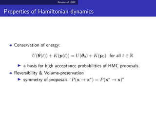
  • 19. Review of HMC Properties of Hamiltonian dynamics Conservation of energy: U(θ(t)) + K(p(t)) = U(θ0) + K(p0) for all t ∈ R a basis for high acceptance probabilities of HMC proposals.
  • 20. Review of HMC Properties of Hamiltonian dynamics Conservation of energy: U(θ(t)) + K(p(t)) = U(θ0) + K(p0) for all t ∈ R a basis for high acceptance probabilities of HMC proposals. Reversibility & Volume-preservation symmetry of proposals “P(x → x∗) = P(x∗ → x)”
  • 21. Turning discrete problems into discontinuous ones Table of Contents 1 Review of HMC 2 Turning discrete problems into discontinuous ones 3 Theory of discontinuous Hamiltonian dynamics 4 Numerical method for discontinuous dynamics 5 Numerical results 6 Results
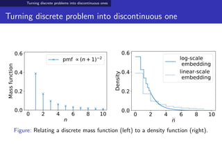
  • 22. Turning discrete problems into discontinuous ones Turning discrete problem into discontinuous one Consider a discrete parameter N ∈ Z+ with a prior πN (·). Map N into a continuous parameter N such that N = n if and only if N ∈ (an, an+1] To match the distribution of N, the corresponding density of N is πN (˜n) = n≥1 πN (n) an+1 − an 1{an < ˜n ≤ an+1}
  • 23. Turning discrete problems into discontinuous ones Turning discrete problem into discontinuous one 0 2 4 6 8 10 n 0.0 0.2 0.4 0.6 Massfunction pmf (n+1) 2 0 2 4 6 8 10 n 0.0 0.2 0.4 0.6 Density log-scale embedding linear-scale embedding Figure: Relating a discrete mass function (left) to a density function (right).
  • 24. Turning discrete problems into discontinuous ones What about more complex discrete spaces? Graphs? Trees? For “momentum” to be useful, we need a notion of direction.
  • 25. Turning discrete problems into discontinuous ones What about more complex discrete spaces? Short answer: I don’t know. (Let me know if you got ideas.) Graphs? Trees? For “momentum” to be useful, we need a notion of direction.
  • 26. Theory of discontinuous Hamiltonian dynamics Table of Contents 1 Review of HMC 2 Turning discrete problems into discontinuous ones 3 Theory of discontinuous Hamiltonian dynamics 4 Numerical method for discontinuous dynamics 5 Numerical results 6 Results
  • 27. Theory of discontinuous Hamiltonian dynamics Theory of discontinuous Hamiltonian dynamics When U(θ) = − log π(θ) is discontinuous, Hamilton’s equations dθ dt = pK(p) dp dt = − θU(θ) (3) becomes a measure-valued differential equation / inclusion. θi U(θ) Figure:
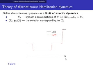
  • 28. Theory of discontinuous Hamiltonian dynamics Theory of discontinuous Hamiltonian dynamics Define discontinuous dynamics as a limit of smooth dynamics: Uδ — smooth approximations of U i.e. limδ→0 Uδ = U. (θδ, pδ)(t) — the solution corresponding to Uδ. θi U(θ) Uδ(θ) Figure:
  • 29. Theory of discontinuous Hamiltonian dynamics Theory of discontinuous Hamiltonian dynamics Define discontinuous dynamics as a limit of smooth dynamics: Uδ — smooth approximations of U i.e. limδ→0 Uδ = U. (θδ, pδ)(t) — the solution corresponding to Uδ. (θ, p)(t) := limδ→0(θδ, pδ)(t). θi U(θ) Uδ(θ) Figure: Example trajectory θ(t) of discontinuous Hamiltonian dynamics.
  • 30. Theory of discontinuous Hamiltonian dynamics Behavior of dynamics at discontinuity When the trajectory θ(t) encounters a discontinuity of U at event time te, the momentum p(t) undergoes an instantaneous change.
  • 31. Theory of discontinuous Hamiltonian dynamics Behavior of dynamics at discontinuity When the trajectory θ(t) encounters a discontinuity of U at event time te, the momentum p(t) undergoes an instantaneous change. The change in p occurs only in the direction of “− θU(θ)”: p(t+ e ) = p(t− e ) − γ ν (θ(te)) where ν(θ) is orthonormal to the discontinuity boundary of U.
  • 32. Theory of discontinuous Hamiltonian dynamics Behavior of dynamics at discontinuity When the trajectory θ(t) encounters a discontinuity of U at event time te, the momentum p(t) undergoes an instantaneous change. The change in p occurs only in the direction of “− θU(θ)”: p(t+ e ) = p(t− e ) − γ ν (θ(te)) where ν(θ) is orthonormal to the discontinuity boundary of U. The scalar γ is determined by the energy conservation principle: K(p(t+ e )) − K(p(t− e )) = U(θ(t− e )) − U(θ(t+ e )) (provided K(p) is convex and K(p) → ∞ as p → ∞).
  • 33. Numerical method for discontinuous dynamics Table of Contents 1 Review of HMC 2 Turning discrete problems into discontinuous ones 3 Theory of discontinuous Hamiltonian dynamics 4 Numerical method for discontinuous dynamics 5 Numerical results 6 Results
  • 34. Numerical method for discontinuous dynamics Dealing with discontinuity
  • 35. Numerical method for discontinuous dynamics Dealing with discontinuity How about ignoring them?
  • 36. Numerical method for discontinuous dynamics Dealing with discontinuity How about ignoring them? Leapfrog integrator completely fails to preserve the energy. i.e. low (or even negligible) acceptance probabilities.
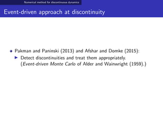
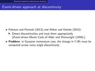
  • 37. Numerical method for discontinuous dynamics Event-driven approach at discontinuity Pakman and Paninski (2013) and Afshar and Domke (2015): Detect discontinuities and treat them appropriately. (Event-driven Monte Carlo of Alder and Wainwright (1959).)
  • 38. Numerical method for discontinuous dynamics Event-driven approach at discontinuity Pakman and Paninski (2013) and Afshar and Domke (2015): Detect discontinuities and treat them appropriately. (Event-driven Monte Carlo of Alder and Wainwright (1959).) Problem: in Gaussian momentum case, the change in U(θ) must be computed across every single discontinuity.
  • 39. Numerical method for discontinuous dynamics Problem with Gaussian momentum & existing approach Say var(N) ≈ 1, 000. Then a Metropolis step N → N ± 1, 000 should have a good chance of acceptance. The numerical method requires 1, 000 density evaluations (ouch!) for a corresponding transition. ΔU ≈ .01 Figure: Conditional distribution of an embedded discrete parameter in the Jolly-Seber example.
  • 40. Numerical method for discontinuous dynamics Laplace momentum: better alternative Consider a Laplace momentum π(p) ∝ i exp(−m−1 i |pi|). The corresponding Hamilton’s equation is dθ dt = m−1 · sign(p), dp dt = − θU(θ)
  • 41. Numerical method for discontinuous dynamics Laplace momentum: better alternative Consider a Laplace momentum π(p) ∝ i exp(−m−1 i |pi|). The corresponding Hamilton’s equation is dθ dt = m−1 · sign(p), dp dt = − θU(θ) Key property: the velocity dθ/dt depends only on the signs of pi’s and not on their magnitudes. This property allows an accurate numerical approximation without keeping track of small changes in pi’s.
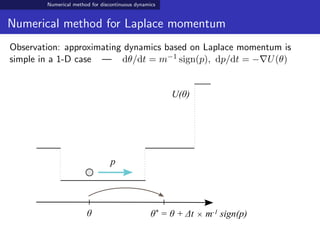
  • 42. Numerical method for discontinuous dynamics Numerical method for Laplace momentum Observation: approximating dynamics based on Laplace momentum is simple in a 1-D case — dθ/dt = m−1 sign(p), dp/dt = − U(θ) θ θ* = θ + Δt × m-1 sign(p) U(θ) p
  • 43. Numerical method for discontinuous dynamics Numerical method for Laplace momentum Observation: approximating dynamics based on Laplace momentum is simple in a 1-D case — dθ/dt = m−1 sign(p), dp/dt = − U(θ) θ θ* = θ + Δt × m-1 sign(p) U(θ) p U(θ*) − U(θ) < K(p) ?
  • 44. Numerical method for discontinuous dynamics Numerical method for Laplace momentum Observation: approximating dynamics based on Laplace momentum is simple in a 1-D case — dθ/dt = m−1 sign(p), dp/dt = − U(θ) θ θ* = θ + Δt × m-1 sign(p) U(θ) U(θ*) − U(θ) = K(p) − K(p*) p*
  • 45. Numerical method for discontinuous dynamics Numerical method for Laplace momentum Observation: approximating dynamics based on Laplace momentum is simple in a 1-D case — dθ/dt = m−1 sign(p), dp/dt = − U(θ) θ θ* U(θ*) − U(θ) p
  • 46. Numerical method for discontinuous dynamics Numerical method for Laplace momentum Observation: approximating dynamics based on Laplace momentum is simple in a 1-D case — dθ/dt = m−1 sign(p), dp/dt = − U(θ) p* ← - p θ* ← θ
  • 47. Numerical method for discontinuous dynamics Coordinate-wise integration for Laplace momentum For θ ∈ Rd, we can split the ODE into its coordinate-wise component: dθi dt = m−1 i sign(pi), dpi dt = −∂θi U(θ), dθ−i dt = dp−i dt = 0 (4)
  • 48. Numerical method for discontinuous dynamics Coordinate-wise integration for Laplace momentum 4 2 0 2 4 2 0 2 4 0 1 2 3 4 5 Figure: Trajectory of a numerical solution via the coordinate-wise integrator.
  • 49. Numerical method for discontinuous dynamics Coordinate-wise integration for Laplace momentum Reversibility preserved by symmetric splitting or randomly permuting the coordinates. We can also use Laplace momentum for discrete parameters and Gaussian momentum for continuous parameters.
  • 50. Numerical method for discontinuous dynamics Properties of discontinuous HMC When using independent Laplace momentum, Proposals are rejection-free thanks to exact energy conservation.1 1 But too big of a stepsize leads to poor mixing.
  • 51. Numerical method for discontinuous dynamics Properties of discontinuous HMC When using independent Laplace momentum, Proposals are rejection-free thanks to exact energy conservation.1 Taking one numerical integration step of DHMC ≡ Variable-at-a-time Metropolis. 1 But too big of a stepsize leads to poor mixing.
  • 52. Numerical method for discontinuous dynamics Properties of discontinuous HMC When using independent Laplace momentum, Proposals are rejection-free thanks to exact energy conservation.1 Taking one numerical integration step of DHMC ≡ Variable-at-a-time Metropolis. When mixing Laplace and Gaussian momentum: Errors in energy is O(∆t2), and hence 1 − O(∆t4) acceptance rate. 1 But too big of a stepsize leads to poor mixing.
  • 53. Numerical results Table of Contents 1 Review of HMC 2 Turning discrete problems into discontinuous ones 3 Theory of discontinuous Hamiltonian dynamics 4 Numerical method for discontinuous dynamics 5 Numerical results 6 Results
  • 54. Numerical results Numerical results: Jolly-Seber (capture-recapture) model Data : the number of marked / unmarked individuals over multiple capture occasions Parameters : population sizes, capture probabilities, survival rates
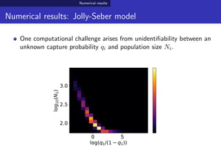
  • 55. Numerical results Numerical results: Jolly-Seber model One computational challenge arises from unidentifiability between an unknown capture probability qi and population size Ni. 0 5 log(q1/(1 q1)) 2.0 2.5 3.0 log10(N1)
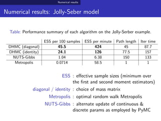
  • 56. Numerical results Numerical results: Jolly-Seber model Table: Performance summary of each algorithm on the Jolly-Serber example. ESS per 100 samples ESS per minute Path length Iter time DHMC (diagonal) 45.5 424 45 87.7 DHMC (identity) 24.1 126 77.5 157 NUTS-Gibbs 1.04 6.38 150 133 Metropolis 0.0714 58.5 1 1 ESS : effective sample sizes (minimum over the first and second moment estimators) diagonal / identity : choice of mass matrix Metropolis : optimal random walk Metropolis NUTS-Gibbs : alternate update of continuous & discrete params as employed by PyMC
  • 57. Numerical results Numerical results: generalized Bayesian inference For a given loss function (y, θ) of interest, a generalized posterior (Bissiri et al., 2016) is given by πpost(θ) ∝ exp − i (yi, θ) πprior(θ) We consider a binary classification with the 0-1 loss (y, θ) = 1{y = sign(x θ)} for y ∈ {−1, 1}.
  • 58. Numerical results Numerical results: generalized Bayesian inference For a given loss function (y, θ) of interest, a generalized posterior (Bissiri et al., 2016) is given by πpost(θ) ∝ exp − i (yi, θ) πprior(θ) We consider a binary classification with the 0-1 loss (y, θ) = 1{y = sign(x θ)} for y ∈ {−1, 1}. 9.2 9.0 8.8 Intercept 0 2 4 6 Density(conditional)
  • 59. Numerical results Numerical results: generalized Bayesian inference Data: semiconductor quality with various sensor measurements Goal: predict faulty products / infer relevant sensor measurements
  • 60. Numerical results Numerical results: generalized Bayesian inference Table: Performance summary on the generalized Bayesian posterior example. ESS per 100 samples ESS per minute Path length Iter time DHMC 26.3 76 25 972 Metropolis 0.00809 (± 0.0018) 0.227 1 1 Variable-at-a-time 0.514 (± 0.039) 39.8 1 36.2 9.2 9.0 8.8 Intercept 0 2 4 6 Density(conditional)
  • 61. Results Table of Contents 1 Review of HMC 2 Turning discrete problems into discontinuous ones 3 Theory of discontinuous Hamiltonian dynamics 4 Numerical method for discontinuous dynamics 5 Numerical results 6 Results
  • 62. Results Summary Hamiltonian dynamics based on Laplace momentum allows an efficient exploration of discontinuous target distributions. Numerical method with exact energy conservation property.
  • 63. Results Future directions Test DHMC on a wider range of applications in the context of a probabilistic programming language. Explore the utility of Laplace momentum as an alternative to Gaussian one. What to do with more complex discrete spaces? Develop notion of directions. Avoid rejections by “swapping” probability between θ and p.
  • 64. Results References Nishimura, A., Dunson, D. and Lu, J. (2017) “Discontinuous Hamiltonian Monte Carlo for sampling discrete parameters,” arXiv:1705.08510. Code available at https://github.com/aki-nishimura/discontinuous-hmc