Quantitative
Methods
for
Lawyers Class #19
Regression Analysis
Part 2
+ 25.39* 1 if region3=true
@ computational
computationallegalstudies.com
professor daniel martin katz danielmartinkatz.com
lexpredict.com slideshare.net/DanielKatz
“We use regression to estimate the unknown effect of changing
one variable over another
regression requires making two assumptions:
1) there is a linear relationship between two variables (i.e. X
and Y)
2) this relationship is additive
(i.e. Y= X1 + X2 + ...+ Xn)
(Note: Additivity applies across terms - as within terms there can be a square,
log, etc.)
Technically, linear regression estimates how much Y changes
when X changes one unit.”
http://dss.princeton.edu/training/
Regression Analysis
Example: After controlling by other factors, are SAT scores
higher in states that spend more money on education?*
Outcome (Y) variable = SAT scores --> variable csat in dataset
Predictor (X) variables
• Per Pupil Expenditures Primary & Secondary (expense)
• % HS of graduates taking SAT (percent)
• Median Household Income (income)
• % adults with HS Diploma (high)
• % adults with College Degree (college)
• Region (region)
Regression Analysis
*Source: search for dataset at http://www.duxbury.com/highered/
Use the file states.dta (educational data for the U.S.).
Getting Started
Lets Begin by Loading it and Use the Head Command
https://s3.amazonaws.com/KatzCloud/states.dta
Getting Started
Use the Summary Command For Additional Information on Each Variable
Bivariate Regression Example
Lets Start Simple:
We Might Hypothesize a Positive Relationship
As Expenditures Go Up
SAT Performances Also Goes Up
Relationship Between Sat Score and Expenditures?
Bivariate Regression Example
It is Certainly NOT Definitive But a Scatterplot is a good
place to start ...
Notice the Nature
of the Relationship
is not what we
would naively
anticipate
It is Certainly NOT Definitive But a Scatterplot is a good
place to start ...
Bivariate Regression Example
It Appears to be
a Negative
Relationship
Notice the Nature
of the Relationship
is not what we
would naively
anticipate
It is Certainly NOT Definitive But a Scatterplot is a good
place to start ...
Bivariate Regression Example
Bivariate
Regression
Notice the -.02155 for
expense which is the
slope of the regression
line shown above
w e j u s t fi t t h e
regression line to this
bivariate relationship
Bivariate Regression
Y = B0 + ( B1 * (X1) )
csat = 1060.7 - (0.022*expense)
For each one-point increase in expense,
SAT scores decrease by 0.022 points.
Bivariate
Regression
Y = B0 + ( B1 * (X1) )
csat = 1060.7 - (0.022*expense)
Look at the
T Stats, P Values
with a Tstat (which is
Z when N>30) of
Greater than 1.96 we
can reject the notion
that the coefficient is
equal to zero
A Brief Word about
Standard Errors
N o t i c e t h a t t h e 9 5 %
Confidence Interval is the Beta
Coefficient ~ Plus or Minus
Two Times the Standard Error
The standard error of the estimate tells us the accuracy to expect from our
prediction -- The standard error of a correlation coefficient is used to determine the
confidence intervals around a true correlation of zero.
look at the Standard Error and you can
obtain the 95% Confidence Interval
1057 + 2(35.5) = ~1127
1057 - 2(35.5) = ~ 987.0
Multivariate
Regression
Now Lets Consider the More Complex Case:
Relationship Between Sat Score and Expenditures/
Variety of other Variables ?
Our Y
Dependent
Variable
Our X Predictors/
Independent Variables
Multivariate Regression
Y = B0 + ( B1 * (X1) ) – ( B2 * (X2) ) + ( B3 * (X3) ) + ( B4 * (X4)) + ( B5 * (X5) ) + ε
csat = 851.56 + 0.003*expense – 2.62*percent + 0.11*income + 1.63*high + 2.03*college + ε
Lets Consider Our
“Beta Coefficients”
Are They
Statistically
Significant?
Look at the
P Value on
“Expense” -
It is no longer
Statistically
Significant
Two Ways to Think
About Significance:
Is the P Value > .05?
Is the Tstat < 1.96?
Variable
Significant
@ .05 Level
expense no
percent yes
income no
high no
college no
intercept yes
Using Our Model to Predict
csat = 851.56 + 0.003*expense – 2.62*percent + 0.11*income + 1.63*high + 2.03*college + ε
Here is our Model:
Using Our Model to Predict
csat = 851.56 + 0.003*expense – 2.62*percent + 0.11*income + 1.63*high + 2.03*college + ε
What if we had a Hypothetical State with the following factors -
• Per Pupil Expenditures Primary & Secondary (expense) - $6000
• % HS of graduates taking SAT (percent) - 20%
• Median Household Income (income) - 33.000
• % adults with HS Diploma (high) - 70%
• % adults with College Degree (college) - 15%
csat = 851.56 + 0.003*(6000) – 2.62*(20) + 0.11*(33.000) + 1.63*(70) + 2.03*(15) + ε
Here is the Predicted SAT SCORE for that STATE:
csat = 851.56 + 18 – 52.4 + 3.63 + 114.1 + 30.45 + ε
csat = 965.34
Here is our Model:
Goodness of Fit
Goodness of Fit
We want to have an idea of how well our regression line fits the data
When we have 1 Independent Variables we are fitting in 2
Dimensional Space
2 Independent Variables we are fitting in 3 Dimensional Space
3 Independent Variables is a 4D Space
Etc.
Note:
Goodness of Fit
Lets look at the correlation structure
First need to do something with this non-numeric column
Goodness of Fit
Lets look at the correlation structure
Need to do something with this non-numeric column
create new version
Goodness of Fit
Lets look at the correlation structure
Need to do something with this non-numeric column
remove the region column
create new version
Goodness of Fit
Lets look at the correlation structure
Need to do something with this non-numeric column
okay all set
remove the region column
create new version
Goodness of Fit
Lets look at the correlation structure
-1
-0.8
-0.6
-0.4
-0.2
0
0.2
0.4
0.6
0.8
1
csat
percent
expense
income
high
college
-0.88
-0.47
-0.47
0.09
-0.37
0.65
0.67
0.14
0.61
0.68
0.31
0.64
0.51
0.72 0.53
1
-0.88
-0.47
-0.47
0.09
-0.37
1
0.65
0.67
0.14
0.61
1
0.68
0.31
0.64
1
0.51
0.72
1
0.53 1
-1 -0.8 -0.6 -0.4 -0.2 0 0.2 0.4 0.6 0.8 1csat
percent
expense
income
high
college
csat
percent
expense
income
high
college
Goodness of Fit
In the 2 Dimensional Case
- the R Squared is Square
of the Correlation
Coefficient
(-0.4663)^2
= 0.2174
Goodness of Fit
These Help Us
Understand the overall fit
of the model
It is the proportion of
variability in a data set
that is accounted for by
the statistical model.
Okay Now Check Out
the Multiple
Regression Case:
R-Squared
Adjusted R-Squared
Goodness of Fit - R2
1-
39351.20
224014.51
R2 = .8243
Goodness of Fit -
The Adjusted R2
R2
= .8243
Adjusted R2
= .8048
Adjusts for the
number of predictors
in the model and the
total sample size
http://www.danielsoper.com/
statcalc3/calc.aspx?id=25
Check it out
at this
website
Goodness of Fit - R2
In regression, the R2
coefficient of determination is a statistical
measure of how well the regression line approximates the real data
points.
An R2
of 1.0 indicates that the regression line perfectly fits the data.
R2
Values closer to 1 indicate a model that better fits the data (there
are important caveats to this so please tread lightly with respect to
R2
)
R2
Values closer to 0 indicate a model that does not fit the data quite
as well
Goodness of Fit - R2
R² does not indicate whether:
* the independent variables are a true cause of the changes in the
dependent variable
* omitted-variable bias exists
* the correct regression was used
* the most appropriate set of independent variables has been chosen
* there is collinearity present in the data on the explanatory variables
* the model might be improved by using transformed versions of the
existing set of independent variables.
Dummy
Variables
Dummy
Variables
dummy variable (also known
as an indicator variable) is
variable that takes the values
(0 or 1) to indicate the
absence or presence of some
categorical effect that may be
expected to shift the outcome
Dummy
Variables
Region can be separated into
4 dummy Variables.
Regions:
1 = West (Base Case)
2 = N. East
3 = South
4 = Midwest
Recoding Dummy Variables
okay but we need to pass these results into something
Recoding Dummy Variables
this will take care of that for you
now we need to bind the two together and pass the
result into a new data set called “states3”
lets take a look at the results ....
Recoding Dummy Variables
okay looks good!
Dummy
Variables
Dummy
Variables
Region can be separated into
4 dummy Variables.
Regions:
1 = West (Base Case)
2 = N. East
3 = South
4 = Midwest
Y = B0 + ( B1 * (X1) ) – ( B2 * (X2) ) + ( B3 * (X3) ) + ( B4 * (X4)) + ( B5 * (X5) ) +
( B6 * (X6) ) + ( B7 * (X7) ) + ( B8 * (X8) ) + ε
csat = 842.59 – 0.002*expense – 3.01*percent – 0.17*income + 1.81*high + 4.67*college +
-34.57*1 if regionWest=true + 34.87* 1 if regionNorthEast=true - 9.18* 1 if regionSouth=true + ε
Dummy
Variables
Take a Look if Region = than the last 3 terms will be turned off
Think of Dummy Variables as Light Switches when
they are on than the associated beta coefficient is on
Y = B0 + ( B1 * (X1) ) – ( B2 * (X2) ) + ( B3 * (X3) ) + ( B4 * (X4)) + ( B5 * (X5) ) +
( B6 * (X6) ) + ( B7 * (X7) ) + ( B8 * (X8) ) + ε
csat = 842.59 – 0.002*expense – 3.01*percent – 0.17*income + 1.81*high + 4.67*college +
-34.57*1 if regionWest=true + 34.87* 1 if regionNorthEast=true - 9.18* 1 if regionSouth=true + ε
Using Our Model to Predict
What if we had a Hypothetical State with the following factors -
• Per Pupil Expenditures Primary & Secondary (expense) - $6000
• % HS of graduates taking SAT (percent) - 20%
• Median Household Income (income) - 33.000
• % adults with HS Diploma (high) - 70%
• % adults with College Degree (college) - 15%
• Midwest State (Region=South)
Please Predict the Mean Score for this Hypothetical State?
Here is our Model:
csat = 849.59 – 0.002*expense – 3.01*percent – 0.17*income + 1.81*high + 4.67*college +
-34.57*1 if regionWest=true + 34.87* 1 if regionNorthEast=true - 9.18* 1 if regionSouth=true + ε
Using Our Model to Predict
What if we had a Hypothetical State with the following factors -
• Per Pupil Expenditures Primary & Secondary (expense) - $6000
• % HS of graduates taking SAT (percent) - 20%
• Median Household Income (income) - 33.000
• % adults with HS Diploma (high) - 70%
• % adults with College Degree (college) - 15%
• Midwest State (Region=South)
Here is our Model:
csat = 849.59 – 0.002*expense – 3.01*percent – 0.17*income + 1.81*high + 4.67*college +
-34.57*1 if regionWest=true + 34.87* 1 if regionNorthEast=true - 9.18* 1 if regionSouth=true + ε
csat = 849.59 – 0.002*(6000) – 3.01*(20) – 0.17*(33.000) + 1.81*(70) + 4.67*(15) +
-34.57*1 if regionWest=true + 34.87* 1 if regionNorthEast=true - 9.18* 1 if regionSouth=true + ε
Using Our Model to Predict
csat = 849.59 – 0.002*(6000) – 3.01*(20) – 0.17*(33.000) + 1.81*(70) + 4.67*(15) +
-34.57*1 if regionWest=true + 34.87* 1 if regionNorthEast=true - 9.18* 1 if regionSouth=true + ε
csat = 849.59 – 0.002*expense – 3.01*percent – 0.17*income + 1.81*high + 4.67*college +
-34.57*1 if regionWest=true + 34.87* 1 if regionNorthEast=true - 9.18* 1 if regionSouth=true + ε
csat = 849.59 – 12 – 60.2 – 5.61 + 126.7 + 70.05 + - 9.18
predicted composite SAT Score = 959.35
Daniel Martin Katz
@ computational
computationallegalstudies.com
lexpredict.com
danielmartinkatz.com
illinois tech - chicago kent college of law@

More Related Content

PDF
Quantitative Methods for Lawyers - Class #12 - Chi Square Distribution and Ch...
PDF
Quantitative Methods for Lawyers - Class #22 - Regression Analysis - Part 1
PDF
Quantitative Methods for Lawyers - Class #14 - R Boot Camp - Part 1 - Profess...
PDF
Quantitative Methods for Lawyers - Bonus Module - Introduction to R, Installi...
PDF
Quantitative Methods for Lawyers - Class #2 - Research Design Part II + Intro...
PDF
Quantitative Methods for Lawyers - Class #6 - Basic Statistics + Probability ...
PDF
Quantitative Methods for Lawyers - Class #3 - Research Design Part III - Pro...
PDF
Quantitative Methods for Lawyers - Class #1 - Why Quantitative Methods + Res...
Quantitative Methods for Lawyers - Class #12 - Chi Square Distribution and Ch...
Quantitative Methods for Lawyers - Class #22 - Regression Analysis - Part 1
Quantitative Methods for Lawyers - Class #14 - R Boot Camp - Part 1 - Profess...
Quantitative Methods for Lawyers - Bonus Module - Introduction to R, Installi...
Quantitative Methods for Lawyers - Class #2 - Research Design Part II + Intro...
Quantitative Methods for Lawyers - Class #6 - Basic Statistics + Probability ...
Quantitative Methods for Lawyers - Class #3 - Research Design Part III - Pro...
Quantitative Methods for Lawyers - Class #1 - Why Quantitative Methods + Res...

What's hot (20)

PDF
Data visualization
PDF
Quantitative Methods for Lawyers - Class #4 - Research Design Part IV - Profe...
PPTX
Random Forest Tutorial | Random Forest in R | Machine Learning | Data Science...
PDF
Linear Regression With R
PDF
Naive Bayes Classifier in Python | Naive Bayes Algorithm | Machine Learning A...
PPTX
Regression (Linear Regression and Logistic Regression) by Akanksha Bali
PPTX
Career in Data Science
PDF
Who is a Data Scientist? | How to become a Data Scientist? | Data Science Cou...
PPTX
Decision Tree and Bayesian Classification
PPTX
Data Science Training | Data Science For Beginners | Data Science With Python...
PPT
Spss introductory session data entry and descriptive stats
PPTX
Decision tree
PPT
Les5e ppt 09
PDF
Quantitative Methods for Lawyers - Class #9 - Bayes Theorem (Part 2), Skewnes...
PPTX
Random Forest and KNN is fun
PDF
Quantitative Methods for Lawyers - Class #10 - Binomial Distributions, Normal...
PPTX
Probability Concept and Bayes Theorem
PDF
Classification and regression trees (cart)
PPT
Linear regression
PDF
2.1 Calculus 2.formulas.pdf.pdf
Data visualization
Quantitative Methods for Lawyers - Class #4 - Research Design Part IV - Profe...
Random Forest Tutorial | Random Forest in R | Machine Learning | Data Science...
Linear Regression With R
Naive Bayes Classifier in Python | Naive Bayes Algorithm | Machine Learning A...
Regression (Linear Regression and Logistic Regression) by Akanksha Bali
Career in Data Science
Who is a Data Scientist? | How to become a Data Scientist? | Data Science Cou...
Decision Tree and Bayesian Classification
Data Science Training | Data Science For Beginners | Data Science With Python...
Spss introductory session data entry and descriptive stats
Decision tree
Les5e ppt 09
Quantitative Methods for Lawyers - Class #9 - Bayes Theorem (Part 2), Skewnes...
Random Forest and KNN is fun
Quantitative Methods for Lawyers - Class #10 - Binomial Distributions, Normal...
Probability Concept and Bayes Theorem
Classification and regression trees (cart)
Linear regression
2.1 Calculus 2.formulas.pdf.pdf
Ad

Similar to Quantitative Methods for Lawyers - Class #19 - Regression Analysis - Part 2 (20)

DOCX
Exercise 29Calculating Simple Linear RegressionSimple linear reg.docx
PDF
Alicia Doyle Lynch Regression in Stata pdf 55 slides.pdf
PDF
Quantitative Methods for Lawyers - Class #20 - Regression Analysis - Part 3
PPT
Regression Analysis.ppt
PPT
Lecture 4
PPT
regration analysishg Annapolis Bhutab.ppt
PPTX
manecohuhuhuhubasicEstimation-1.pptx
PPTX
Correlation & Regression.pptx
PDF
Quantitative Methods for Lawyers - Class #21 - Regression Analysis - Part 4
PPT
Unit 8 lesson 1
DOCX
For this assignment, use the aschooltest.sav dataset.The d
PPTX
Regression analysis
PPTX
An Introduction to Regression Models: Linear and Logistic approaches
PPTX
Applied Stats for Real-Life Decisions.pptx
PDF
Materi_Business_Intelligence_1.pdf
PPTX
Regression Analysis presentation by Al Arizmendez and Cathryn Lottier
PPTX
Recep maz msb 701 quantitative analysis for managers
PPTX
Recep maz msb 701 quantitative analysis for managers
PPT
Powerpoint2.reg
Exercise 29Calculating Simple Linear RegressionSimple linear reg.docx
Alicia Doyle Lynch Regression in Stata pdf 55 slides.pdf
Quantitative Methods for Lawyers - Class #20 - Regression Analysis - Part 3
Regression Analysis.ppt
Lecture 4
regration analysishg Annapolis Bhutab.ppt
manecohuhuhuhubasicEstimation-1.pptx
Correlation & Regression.pptx
Quantitative Methods for Lawyers - Class #21 - Regression Analysis - Part 4
Unit 8 lesson 1
For this assignment, use the aschooltest.sav dataset.The d
Regression analysis
An Introduction to Regression Models: Linear and Logistic approaches
Applied Stats for Real-Life Decisions.pptx
Materi_Business_Intelligence_1.pdf
Regression Analysis presentation by Al Arizmendez and Cathryn Lottier
Recep maz msb 701 quantitative analysis for managers
Powerpoint2.reg
Ad

More from Daniel Katz (20)

PDF
Legal Analytics versus Empirical Legal Studies - or - Causal Inference vs Pre...
PDF
Can Law Librarians Help Law Become More Data Driven ? An Open Question in Ne...
DOCX
Why We Are Open Sourcing ContraxSuite and Some Thoughts About Legal Tech and ...
PDF
Fin (Legal) Tech – Law’s Future from Finance’s Past (Some Thoughts About the ...
PDF
Exploring the Physical Properties of Regulatory Ecosystems - Professors Danie...
PDF
Law + Complexity & Prediction: Toward a Characterization of Legal Systems as ...
PDF
Building Your Personal (Legal) Brand - Some Thoughts for Law Students and Oth...
PDF
Measure Twice, Cut Once - Solving the Legal Profession Biggest Challenges Tog...
PDF
Artificial Intelligence and Law - 
A Primer
PDF
Machine Learning as a Service: #MLaaS, Open Source and the Future of (Legal) ...
PDF
Technology, Data and Computation Session @ The World Bank - Law, Justice, and...
PDF
LexPredict - Empowering the Future of Legal Decision Making
PDF
{Law, Tech, Design, Delivery} Observations Regarding Innovation in the Legal ...
PDF
Legal Analytics Course - Class 11 - Network Analysis and Law - Professors Dan...
PDF
Legal Analytics Course - Class 12 - Data Preprocessing using dPlyR - Professo...
PDF
Legal Analytics Course - Class 10 - Information Visualization + DataViz in R ...
PDF
Legal Analytics Course - Class #4 - Github and RMarkdown Tutorial - Professor...
PDF
Legal Analytics Course - Class 9 - Clustering Algorithms (K-Means & Hierarch...
PDF
Legal Analytics Course - Class 8 - Introduction to Random Forests and Ensembl...
PDF
Legal Analytics Course - Class 7 - Binary Classification with Decision Tree L...
Legal Analytics versus Empirical Legal Studies - or - Causal Inference vs Pre...
Can Law Librarians Help Law Become More Data Driven ? An Open Question in Ne...
Why We Are Open Sourcing ContraxSuite and Some Thoughts About Legal Tech and ...
Fin (Legal) Tech – Law’s Future from Finance’s Past (Some Thoughts About the ...
Exploring the Physical Properties of Regulatory Ecosystems - Professors Danie...
Law + Complexity & Prediction: Toward a Characterization of Legal Systems as ...
Building Your Personal (Legal) Brand - Some Thoughts for Law Students and Oth...
Measure Twice, Cut Once - Solving the Legal Profession Biggest Challenges Tog...
Artificial Intelligence and Law - 
A Primer
Machine Learning as a Service: #MLaaS, Open Source and the Future of (Legal) ...
Technology, Data and Computation Session @ The World Bank - Law, Justice, and...
LexPredict - Empowering the Future of Legal Decision Making
{Law, Tech, Design, Delivery} Observations Regarding Innovation in the Legal ...
Legal Analytics Course - Class 11 - Network Analysis and Law - Professors Dan...
Legal Analytics Course - Class 12 - Data Preprocessing using dPlyR - Professo...
Legal Analytics Course - Class 10 - Information Visualization + DataViz in R ...
Legal Analytics Course - Class #4 - Github and RMarkdown Tutorial - Professor...
Legal Analytics Course - Class 9 - Clustering Algorithms (K-Means & Hierarch...
Legal Analytics Course - Class 8 - Introduction to Random Forests and Ensembl...
Legal Analytics Course - Class 7 - Binary Classification with Decision Tree L...

Recently uploaded (20)

PPTX
Human Rights as per Indian Constitution.
PPTX
Evolution of First Amendment Jurisprudence.pptx
PDF
Legal Strategics for Startup Success Contracts.pdf
PPTX
Philippine Politics and Governance - Lesson 10 - The Executive Branch
PDF
Black And Deep Peach Geometric Legal Advisor Firm Presentation.pdf
PPT
Role of trustees in EC Competition Law.ppt
PPTX
Rights of the Accused Presentation CLEPI
DOCX
CHAPTER 1 OBLICON.............................
PPT
Gender sensitivity and fair language implementation
PPTX
white collar crime .pptx power function and punishment
PPT
2025 KATARUNGANG PAMBARANGAY LECTURE.ppt
PPTX
PRODUCT LIABILITY AMID TECHNOLOGICAL DISRUPTION_ ABATING THE SURGE OF DIGITAL...
PDF
Palghar-286Nilemore-VoterList-Aug25-1.pdf
PPTX
lecture 5.pptx on family law notes well detailed
PPTX
Unit 2The Making of India's Constitution
PDF
2022CH12581 - Civil Rights vs Morzak, Harrison, Chrisman et al. (Cook County,...
PPTX
Legal drafting is the most important instrument of legal communication. The s...
PDF
Divorce Attorney Chicago – Guiding You Through Every Step
PPTX
Sexual Harassment Prevention training class
Human Rights as per Indian Constitution.
Evolution of First Amendment Jurisprudence.pptx
Legal Strategics for Startup Success Contracts.pdf
Philippine Politics and Governance - Lesson 10 - The Executive Branch
Black And Deep Peach Geometric Legal Advisor Firm Presentation.pdf
Role of trustees in EC Competition Law.ppt
Rights of the Accused Presentation CLEPI
CHAPTER 1 OBLICON.............................
Gender sensitivity and fair language implementation
white collar crime .pptx power function and punishment
2025 KATARUNGANG PAMBARANGAY LECTURE.ppt
PRODUCT LIABILITY AMID TECHNOLOGICAL DISRUPTION_ ABATING THE SURGE OF DIGITAL...
Palghar-286Nilemore-VoterList-Aug25-1.pdf
lecture 5.pptx on family law notes well detailed
Unit 2The Making of India's Constitution
2022CH12581 - Civil Rights vs Morzak, Harrison, Chrisman et al. (Cook County,...
Legal drafting is the most important instrument of legal communication. The s...
Divorce Attorney Chicago – Guiding You Through Every Step
Sexual Harassment Prevention training class

Quantitative Methods for Lawyers - Class #19 - Regression Analysis - Part 2

  • 1. Quantitative Methods for Lawyers Class #19 Regression Analysis Part 2 + 25.39* 1 if region3=true @ computational computationallegalstudies.com professor daniel martin katz danielmartinkatz.com lexpredict.com slideshare.net/DanielKatz
  • 2. “We use regression to estimate the unknown effect of changing one variable over another regression requires making two assumptions: 1) there is a linear relationship between two variables (i.e. X and Y) 2) this relationship is additive (i.e. Y= X1 + X2 + ...+ Xn) (Note: Additivity applies across terms - as within terms there can be a square, log, etc.) Technically, linear regression estimates how much Y changes when X changes one unit.” http://dss.princeton.edu/training/ Regression Analysis
  • 3. Example: After controlling by other factors, are SAT scores higher in states that spend more money on education?* Outcome (Y) variable = SAT scores --> variable csat in dataset Predictor (X) variables • Per Pupil Expenditures Primary & Secondary (expense) • % HS of graduates taking SAT (percent) • Median Household Income (income) • % adults with HS Diploma (high) • % adults with College Degree (college) • Region (region) Regression Analysis *Source: search for dataset at http://www.duxbury.com/highered/ Use the file states.dta (educational data for the U.S.).
  • 4. Getting Started Lets Begin by Loading it and Use the Head Command https://s3.amazonaws.com/KatzCloud/states.dta
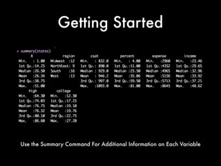
  • 5. Getting Started Use the Summary Command For Additional Information on Each Variable
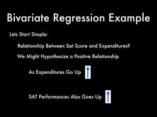
  • 6. Bivariate Regression Example Lets Start Simple: We Might Hypothesize a Positive Relationship As Expenditures Go Up SAT Performances Also Goes Up Relationship Between Sat Score and Expenditures?
  • 7. Bivariate Regression Example It is Certainly NOT Definitive But a Scatterplot is a good place to start ...
  • 8. Notice the Nature of the Relationship is not what we would naively anticipate It is Certainly NOT Definitive But a Scatterplot is a good place to start ... Bivariate Regression Example
  • 9. It Appears to be a Negative Relationship Notice the Nature of the Relationship is not what we would naively anticipate It is Certainly NOT Definitive But a Scatterplot is a good place to start ... Bivariate Regression Example
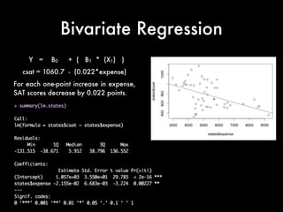
  • 10. Bivariate Regression Notice the -.02155 for expense which is the slope of the regression line shown above w e j u s t fi t t h e regression line to this bivariate relationship
  • 11. Bivariate Regression Y = B0 + ( B1 * (X1) ) csat = 1060.7 - (0.022*expense) For each one-point increase in expense, SAT scores decrease by 0.022 points.
  • 12. Bivariate Regression Y = B0 + ( B1 * (X1) ) csat = 1060.7 - (0.022*expense) Look at the T Stats, P Values with a Tstat (which is Z when N>30) of Greater than 1.96 we can reject the notion that the coefficient is equal to zero
  • 13. A Brief Word about Standard Errors N o t i c e t h a t t h e 9 5 % Confidence Interval is the Beta Coefficient ~ Plus or Minus Two Times the Standard Error The standard error of the estimate tells us the accuracy to expect from our prediction -- The standard error of a correlation coefficient is used to determine the confidence intervals around a true correlation of zero. look at the Standard Error and you can obtain the 95% Confidence Interval 1057 + 2(35.5) = ~1127 1057 - 2(35.5) = ~ 987.0
  • 15. Now Lets Consider the More Complex Case: Relationship Between Sat Score and Expenditures/ Variety of other Variables ? Our Y Dependent Variable Our X Predictors/ Independent Variables Multivariate Regression
  • 16. Y = B0 + ( B1 * (X1) ) – ( B2 * (X2) ) + ( B3 * (X3) ) + ( B4 * (X4)) + ( B5 * (X5) ) + ε csat = 851.56 + 0.003*expense – 2.62*percent + 0.11*income + 1.63*high + 2.03*college + ε
  • 17. Lets Consider Our “Beta Coefficients” Are They Statistically Significant? Look at the P Value on “Expense” - It is no longer Statistically Significant
  • 18. Two Ways to Think About Significance: Is the P Value > .05? Is the Tstat < 1.96? Variable Significant @ .05 Level expense no percent yes income no high no college no intercept yes
  • 19. Using Our Model to Predict
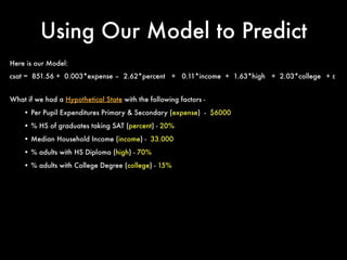
  • 20. Using Our Model to Predict csat = 851.56 + 0.003*expense – 2.62*percent + 0.11*income + 1.63*high + 2.03*college + ε Here is our Model:
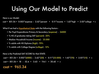
  • 21. Using Our Model to Predict csat = 851.56 + 0.003*expense – 2.62*percent + 0.11*income + 1.63*high + 2.03*college + ε What if we had a Hypothetical State with the following factors - • Per Pupil Expenditures Primary & Secondary (expense) - $6000 • % HS of graduates taking SAT (percent) - 20% • Median Household Income (income) - 33.000 • % adults with HS Diploma (high) - 70% • % adults with College Degree (college) - 15% Here is our Model:
  • 22. Using Our Model to Predict csat = 851.56 + 0.003*expense – 2.62*percent + 0.11*income + 1.63*high + 2.03*college + ε What if we had a Hypothetical State with the following factors - • Per Pupil Expenditures Primary & Secondary (expense) - $6000 • % HS of graduates taking SAT (percent) - 20% • Median Household Income (income) - 33.000 • % adults with HS Diploma (high) - 70% • % adults with College Degree (college) - 15% csat = 851.56 + 0.003*(6000) – 2.62*(20) + 0.11*(33.000) + 1.63*(70) + 2.03*(15) + ε Here is the Predicted SAT SCORE for that STATE: csat = 851.56 + 18 – 52.4 + 3.63 + 114.1 + 30.45 + ε csat = 965.34 Here is our Model:
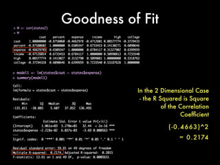
  • 24. Goodness of Fit We want to have an idea of how well our regression line fits the data When we have 1 Independent Variables we are fitting in 2 Dimensional Space 2 Independent Variables we are fitting in 3 Dimensional Space 3 Independent Variables is a 4D Space Etc. Note:
  • 25. Goodness of Fit Lets look at the correlation structure First need to do something with this non-numeric column
  • 26. Goodness of Fit Lets look at the correlation structure Need to do something with this non-numeric column create new version
  • 27. Goodness of Fit Lets look at the correlation structure Need to do something with this non-numeric column remove the region column create new version
  • 28. Goodness of Fit Lets look at the correlation structure Need to do something with this non-numeric column okay all set remove the region column create new version
  • 29. Goodness of Fit Lets look at the correlation structure -1 -0.8 -0.6 -0.4 -0.2 0 0.2 0.4 0.6 0.8 1 csat percent expense income high college -0.88 -0.47 -0.47 0.09 -0.37 0.65 0.67 0.14 0.61 0.68 0.31 0.64 0.51 0.72 0.53 1 -0.88 -0.47 -0.47 0.09 -0.37 1 0.65 0.67 0.14 0.61 1 0.68 0.31 0.64 1 0.51 0.72 1 0.53 1 -1 -0.8 -0.6 -0.4 -0.2 0 0.2 0.4 0.6 0.8 1csat percent expense income high college csat percent expense income high college
  • 30. Goodness of Fit In the 2 Dimensional Case - the R Squared is Square of the Correlation Coefficient (-0.4663)^2 = 0.2174
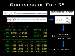
  • 31. Goodness of Fit These Help Us Understand the overall fit of the model It is the proportion of variability in a data set that is accounted for by the statistical model. Okay Now Check Out the Multiple Regression Case: R-Squared Adjusted R-Squared
  • 32. Goodness of Fit - R2 1- 39351.20 224014.51 R2 = .8243
  • 33. Goodness of Fit - The Adjusted R2 R2 = .8243 Adjusted R2 = .8048 Adjusts for the number of predictors in the model and the total sample size http://www.danielsoper.com/ statcalc3/calc.aspx?id=25 Check it out at this website
  • 34. Goodness of Fit - R2 In regression, the R2 coefficient of determination is a statistical measure of how well the regression line approximates the real data points. An R2 of 1.0 indicates that the regression line perfectly fits the data. R2 Values closer to 1 indicate a model that better fits the data (there are important caveats to this so please tread lightly with respect to R2 ) R2 Values closer to 0 indicate a model that does not fit the data quite as well
  • 35. Goodness of Fit - R2 R² does not indicate whether: * the independent variables are a true cause of the changes in the dependent variable * omitted-variable bias exists * the correct regression was used * the most appropriate set of independent variables has been chosen * there is collinearity present in the data on the explanatory variables * the model might be improved by using transformed versions of the existing set of independent variables.
  • 37. Dummy Variables dummy variable (also known as an indicator variable) is variable that takes the values (0 or 1) to indicate the absence or presence of some categorical effect that may be expected to shift the outcome
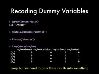
  • 38. Dummy Variables Region can be separated into 4 dummy Variables. Regions: 1 = West (Base Case) 2 = N. East 3 = South 4 = Midwest
  • 40. Recoding Dummy Variables okay but we need to pass these results into something
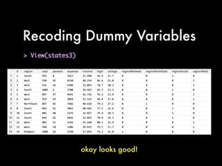
  • 41. Recoding Dummy Variables this will take care of that for you now we need to bind the two together and pass the result into a new data set called “states3” lets take a look at the results ....
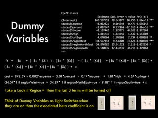
  • 44. Dummy Variables Region can be separated into 4 dummy Variables. Regions: 1 = West (Base Case) 2 = N. East 3 = South 4 = Midwest Y = B0 + ( B1 * (X1) ) – ( B2 * (X2) ) + ( B3 * (X3) ) + ( B4 * (X4)) + ( B5 * (X5) ) + ( B6 * (X6) ) + ( B7 * (X7) ) + ( B8 * (X8) ) + ε csat = 842.59 – 0.002*expense – 3.01*percent – 0.17*income + 1.81*high + 4.67*college + -34.57*1 if regionWest=true + 34.87* 1 if regionNorthEast=true - 9.18* 1 if regionSouth=true + ε
  • 45. Dummy Variables Take a Look if Region = than the last 3 terms will be turned off Think of Dummy Variables as Light Switches when they are on than the associated beta coefficient is on Y = B0 + ( B1 * (X1) ) – ( B2 * (X2) ) + ( B3 * (X3) ) + ( B4 * (X4)) + ( B5 * (X5) ) + ( B6 * (X6) ) + ( B7 * (X7) ) + ( B8 * (X8) ) + ε csat = 842.59 – 0.002*expense – 3.01*percent – 0.17*income + 1.81*high + 4.67*college + -34.57*1 if regionWest=true + 34.87* 1 if regionNorthEast=true - 9.18* 1 if regionSouth=true + ε
  • 46. Using Our Model to Predict
  • 47. Using Our Model to Predict What if we had a Hypothetical State with the following factors - • Per Pupil Expenditures Primary & Secondary (expense) - $6000 • % HS of graduates taking SAT (percent) - 20% • Median Household Income (income) - 33.000 • % adults with HS Diploma (high) - 70% • % adults with College Degree (college) - 15% • Midwest State (Region=South) Please Predict the Mean Score for this Hypothetical State? Here is our Model: csat = 849.59 – 0.002*expense – 3.01*percent – 0.17*income + 1.81*high + 4.67*college + -34.57*1 if regionWest=true + 34.87* 1 if regionNorthEast=true - 9.18* 1 if regionSouth=true + ε
  • 48. Using Our Model to Predict What if we had a Hypothetical State with the following factors - • Per Pupil Expenditures Primary & Secondary (expense) - $6000 • % HS of graduates taking SAT (percent) - 20% • Median Household Income (income) - 33.000 • % adults with HS Diploma (high) - 70% • % adults with College Degree (college) - 15% • Midwest State (Region=South) Here is our Model: csat = 849.59 – 0.002*expense – 3.01*percent – 0.17*income + 1.81*high + 4.67*college + -34.57*1 if regionWest=true + 34.87* 1 if regionNorthEast=true - 9.18* 1 if regionSouth=true + ε csat = 849.59 – 0.002*(6000) – 3.01*(20) – 0.17*(33.000) + 1.81*(70) + 4.67*(15) + -34.57*1 if regionWest=true + 34.87* 1 if regionNorthEast=true - 9.18* 1 if regionSouth=true + ε
  • 49. Using Our Model to Predict csat = 849.59 – 0.002*(6000) – 3.01*(20) – 0.17*(33.000) + 1.81*(70) + 4.67*(15) + -34.57*1 if regionWest=true + 34.87* 1 if regionNorthEast=true - 9.18* 1 if regionSouth=true + ε csat = 849.59 – 0.002*expense – 3.01*percent – 0.17*income + 1.81*high + 4.67*college + -34.57*1 if regionWest=true + 34.87* 1 if regionNorthEast=true - 9.18* 1 if regionSouth=true + ε csat = 849.59 – 12 – 60.2 – 5.61 + 126.7 + 70.05 + - 9.18 predicted composite SAT Score = 959.35
  • 50. Daniel Martin Katz @ computational computationallegalstudies.com lexpredict.com danielmartinkatz.com illinois tech - chicago kent college of law@