Regression and Classification with R

cation with R
Yanchang Zhao
http://www.RDataMining.com
30 September 2014
1 / 44

Outline
Introduction
Linear Regression
Generalized Linear Regression
Decision Trees with Package party
Decision Trees with Package rpart
Random Forest
Online Resources
2 / 44

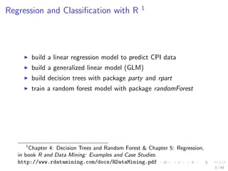
cation with R 1
I build a linear regression model to predict CPI data
I build a generalized linear model (GLM)
I build decision trees with package party and rpart
I train a random forest model with package randomForest
1Chapter 4: Decision Trees and Random Forest & Chapter 5: Regression,
in book R and Data Mining: Examples and Case Studies.
http://www.rdatamining.com/docs/RDataMining.pdf
3 / 44

Regression
I Regression is to build a function of independent variables (also
known as predictors) to predict a dependent variable (also
called response).
I For example, banks assess the risk of home-loan applicants
based on their age, income, expenses, occupation, number of
dependents, total credit limit, etc.
I linear regression models
I generalized linear models (GLM)
4 / 44

Outline
Introduction
Linear Regression
Random Forest
Online Resources
5 / 44

Linear Regression
I Linear regression is to predict response with a linear function
of predictors as follows:
y = c0 + c1x1 + c2x2 + + ckxk ;
where x1; x2; ; xk are predictors and y is the response to
predict.
I linear regression with function lm()
I the Australian CPI (Consumer Price Index) data: quarterly
CPIs from 2008 to 2010 2
2From Australian Bureau of Statistics, http://www.abs.gov.au.
6 / 44

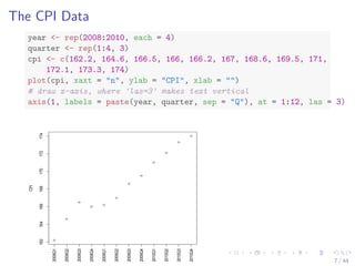
The CPI Data
year - rep(2008:2010, each = 4)
quarter - rep(1:4, 3)
cpi - c(162.2, 164.6, 166.5, 166, 166.2, 167, 168.6, 169.5, 171,
172.1, 173.3, 174)
plot(cpi, xaxt = n, ylab = CPI, xlab = )
# draw x-axis, where 'las=3' makes text vertical
axis(1, labels = paste(year, quarter, sep = Q), at = 1:12, las = 3)
162 164 166 168 170 172 174
CPI
2008Q1
2008Q2
2008Q3
2008Q4
2009Q1
2009Q2
2009Q3
2009Q4
2010Q1
2010Q2
2010Q3
2010Q4
7 / 44

Linear Regression
## correlation between CPI and year / quarter
cor(year, cpi)
## [1] 0.9096
cor(quarter, cpi)
## [1] 0.3738
## build a linear regression model with function lm()
fit - lm(cpi ~ year + quarter)
fit
##
## Call:
## lm(formula = cpi ~ year + quarter)
##
## Coefficients:
## (Intercept) year quarter
## -7644.49 3.89 1.17
8 / 44

With the above linear model, CPI is calculated as
cpi = c0 + c1 year + c2 quarter;
where c0, c1 and c2 are coecients from model fit.
What will the CPI be in 2011?
cpi2011 - fit$coefficients[[1]] +
fit$coefficients[[2]] * 2011 +
fit$coefficients[[3]] * (1:4)
cpi2011
## [1] 174.4 175.6 176.8 177.9
9 / 44

With the above linear model, CPI is calculated as
cpi = c0 + c1 year + c2 quarter;
where c0, c1 and c2 are coecients from model fit.
What will the CPI be in 2011?
cpi2011 - fit$coefficients[[1]] +
fit$coefficients[[2]] * 2011 +
fit$coefficients[[3]] * (1:4)
cpi2011
## [1] 174.4 175.6 176.8 177.9
An easier way is to use function predict().
9 / 44

More details of the model can be obtained with the code below.
attributes(fit)
## $names
## [1] coefficients residuals effects
## [4] rank fitted.values assign
## [7] qr df.residual xlevels
## [10] call terms model
##
## $class
## [1] lm
fit$coefficients
## (Intercept) year quarter
## -7644.488 3.888 1.167
10 / 44

Function residuals(): dierences between observed values and

tted values
# differences between observed values and fitted values
residuals(fit)
## 1 2 3 4 5 6 ...
## -0.57917 0.65417 1.38750 -0.27917 -0.46667 -0.83333 -0.40...
## 8 9 10 11 12
## -0.66667 0.44583 0.37917 0.41250 -0.05417
summary(fit)
##
## Call:
## lm(formula = cpi ~ year + quarter)
##
## Residuals:
## Min 1Q Median 3Q Max
## -0.833 -0.495 -0.167 0.421 1.387
##
## Coefficients:
## Estimate Std. Error t value Pr(|t|)
## (Intercept) -7644.488 518.654 -14.74 1.3e-07 ***
## year 3.888 0.258 15.06 1.1e-07 ***
11 / 44

3D Plot of the Fitted Model
library(scatterplot3d)
s3d - scatterplot3d(year, quarter, cpi, highlight.3d = T, type = h,
lab = c(2, 3)) # lab: number of tickmarks on x-/y-axes
s3d$plane3d(fit) # draws the fitted plane
160 165 170 175
2008 2009 2010
1
2
3
4
year
quarter
cpi
12 / 44

Prediction of CPIs in 2011
data2011 - data.frame(year = 2011, quarter = 1:4)
cpi2011 - predict(fit, newdata = data2011)
style - c(rep(1, 12), rep(2, 4))
plot(c(cpi, cpi2011), xaxt = n, ylab = CPI, xlab = , pch = style,
col = style)
axis(1, at = 1:16, las = 3, labels = c(paste(year, quarter, sep = Q),
2011Q1, 2011Q2, 2011Q3, 2011Q4))
165 170 175
CPI
2008Q1
2008Q2
2008Q3
2008Q4
2009Q1
2009Q2
2009Q3
2009Q4
2010Q1
2010Q2
2010Q3
2010Q4
2011Q1
2011Q2
2011Q3
2011Q4
13 / 44

Outline
Introduction
Linear Regression
Random Forest
Online Resources
14 / 44

Generalized Linear Model (GLM)
I Generalizes linear regression by allowing the linear model to be
related to the response variable via a link function and
allowing the magnitude of the variance of each measurement
to be a function of its predicted value
I Uni

es various other statistical models, including linear
regression, logistic regression and Poisson regression
I Function glm():

ts generalized linear models, speci

ed by
giving a symbolic description of the linear predictor and a
description of the error distribution
15 / 44

Build a Generalized Linear Model
data(bodyfat, package=TH.data)
myFormula - DEXfat ~ age + waistcirc + hipcirc + elbowbreadth +
kneebreadth
bodyfat.glm - glm(myFormula, family = gaussian(log), data = bodyfat)
summary(bodyfat.glm)
##
## Call:
## glm(formula = myFormula, family = gaussian(log), data = b...
##
## Deviance Residuals:
## Min 1Q Median 3Q Max
## -11.569 -3.006 0.127 2.831 10.097
##
## Coefficients:
## Estimate Std. Error t value Pr(|t|)
## (Intercept) 0.73429 0.30895 2.38 0.0204 *
## age 0.00213 0.00145 1.47 0.1456
## waistcirc 0.01049 0.00248 4.23 7.4e-05 ***
## hipcirc 0.00970 0.00323 3.00 0.0038 **
## elbowbreadth 0.00235 0.04569 0.05 0.9590
## kneebreadth 0.06319 0.02819 2.24 0.0284 *
16 / 44

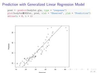
Prediction with Generalized Linear Regression Model
pred - predict(bodyfat.glm, type = response)
plot(bodyfat$DEXfat, pred, xlab = Observed, ylab = Prediction)
abline(a = 0, b = 1)
10 20 30 40 50 60
20 30 40 50
Observed
Prediction
17 / 44

Outline
Introduction
Linear Regression
Random Forest
Online Resources
18 / 44

The iris Data
str(iris)
## 'data.frame': 150 obs. of 5 variables:
## $ Sepal.Length: num 5.1 4.9 4.7 4.6 5 5.4 4.6 5 4.4 4.9 ...
## $ Sepal.Width : num 3.5 3 3.2 3.1 3.6 3.9 3.4 3.4 2.9 3.1...
## $ Petal.Length: num 1.4 1.4 1.3 1.5 1.4 1.7 1.4 1.5 1.4 1...
## $ Petal.Width : num 0.2 0.2 0.2 0.2 0.2 0.4 0.3 0.2 0.2 0...
## $ Species : Factor w/ 3 levels setosa,versicolor,....
# split data into two subsets: training (70%) and test (30%); set
# a fixed random seed to make results reproducible
set.seed(1234)
ind - sample(2, nrow(iris), replace = TRUE, prob = c(0.7, 0.3))
train.data - iris[ind == 1, ]
test.data - iris[ind == 2, ]
19 / 44

Build a ctree
I Control the training of decision trees: MinSplit, MinBusket,
MaxSurrogate and MaxDepth
I Target variable: Species
I Independent variables: all other variables
library(party)
myFormula - Species ~ Sepal.Length + Sepal.Width + Petal.Length +
Petal.Width
iris_ctree - ctree(myFormula, data = train.data)
# check the prediction
table(predict(iris_ctree), train.data$Species)
##
## setosa versicolor virginica
## setosa 40 0 0
## versicolor 0 37 3
## virginica 0 1 31
20 / 44

Print ctree
print(iris_ctree)
##
## Conditional inference tree with 4 terminal nodes
##
## Response: Species
## Inputs: Sepal.Length, Sepal.Width, Petal.Length, Petal.Width
## Number of observations: 112
##
## 1) Petal.Length = 1.9; criterion = 1, statistic = 104.643
## 2)* weights = 40
## 1) Petal.Length 1.9
## 3) Petal.Width = 1.7; criterion = 1, statistic = 48.939
## 4) Petal.Length = 4.4; criterion = 0.974, statistic = ...
## 5)* weights = 21
## 4) Petal.Length 4.4
## 6)* weights = 19
## 3) Petal.Width 1.7
## 7)* weights = 32
21 / 44

plot(iris_ctree)
1
Petal.Length
p 0.001
£ 1.9 1.9
Node 2 (n = 40)
setosa
1
0.8
0.6
0.4
0.2
0
3
Petal.Width
p 0.001
£ 1.7 1.7
4
Petal.Length
p = 0.026
£ 4.4 4.4
Node 5 (n = 21)
setosa
1
0.8
0.6
0.4
0.2
0
Node 6 (n = 19)
setosa
1
0.8
0.6
0.4
0.2
0
Node 7 (n = 32)
setosa
1
0.8
0.6
0.4
0.2
0
22 / 44

plot(iris_ctree, type = simple)
1
Petal.Length
p 0.001
£ 1.9 1.9
2
n = 40
y = (1, 0, 0)
3
Petal.Width
p 0.001
£ 1.7 1.7
4
Petal.Length
p = 0.026
£ 4.4 4.4
5
n = 21
y = (0, 1, 0)
6
n = 19
y = (0, 0.842, 0.158)
7
n = 32
y = (0, 0.031, 0.969)
23 / 44

Test
# predict on test data
testPred - predict(iris_ctree, newdata = test.data)
table(testPred, test.data$Species)
##
## testPred setosa versicolor virginica
## setosa 10 0 0
## virginica 0 0 14
24 / 44

Outline
Introduction
Linear Regression
Random Forest
Online Resources
25 / 44

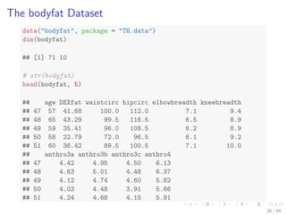
The bodyfat Dataset
data(bodyfat, package = TH.data)
dim(bodyfat)
## [1] 71 10
# str(bodyfat)
head(bodyfat, 5)
## age DEXfat waistcirc hipcirc elbowbreadth kneebreadth
## 47 57 41.68 100.0 112.0 7.1 9.4
## 48 65 43.29 99.5 116.5 6.5 8.9
## 49 59 35.41 96.0 108.5 6.2 8.9
## 50 58 22.79 72.0 96.5 6.1 9.2
## 51 60 36.42 89.5 100.5 7.1 10.0
## anthro3a anthro3b anthro3c anthro4
## 47 4.42 4.95 4.50 6.13
## 48 4.63 5.01 4.48 6.37
## 49 4.12 4.74 4.60 5.82
## 50 4.03 4.48 3.91 5.66
## 51 4.24 4.68 4.15 5.91
26 / 44

Train a Decision Tree with Package rpart
# split into training and test subsets
set.seed(1234)
ind - sample(2, nrow(bodyfat), replace=TRUE, prob=c(0.7, 0.3))
bodyfat.train - bodyfat[ind==1,]
bodyfat.test - bodyfat[ind==2,]
# train a decision tree
library(rpart)
myFormula - DEXfat ~ age + waistcirc + hipcirc + elbowbreadth +
kneebreadth
bodyfat_rpart - rpart(myFormula, data = bodyfat.train,
control = rpart.control(minsplit = 10))
# print(bodyfat_rpart$cptable)
print(bodyfat_rpart)
plot(bodyfat_rpart)
text(bodyfat_rpart, use.n=T)
27 / 44

The rpart Tree
## n= 56
##
## node), split, n, deviance, yval
## * denotes terminal node
##
## 1) root 56 7265.0000 30.95
## 2) waistcirc 88.4 31 960.5000 22.56
## 4) hipcirc 96.25 14 222.3000 18.41
## 8) age 60.5 9 66.8800 16.19 *
## 9) age=60.5 5 31.2800 22.41 *
## 5) hipcirc=96.25 17 299.6000 25.97
## 10) waistcirc 77.75 6 30.7300 22.32 *
## 11) waistcirc=77.75 11 145.7000 27.96
## 22) hipcirc 99.5 3 0.2569 23.75 *
## 23) hipcirc=99.5 8 72.2900 29.54 *
## 3) waistcirc=88.4 25 1417.0000 41.35
## 6) waistcirc 104.8 18 330.6000 38.09
## 12) hipcirc 109.9 9 69.0000 34.38 *
## 13) hipcirc=109.9 9 13.0800 41.81 *
## 7) waistcirc=104.8 7 404.3000 49.73 *
28 / 44

The rpart Tree
waistcir|c 88.4
hipcirc 96.25
age 60.5 waistcirc 77.75
hipcirc 99.5
waistcirc 104.8
2e+01 hipcirc 109.9
n=9
2e+01
n=5 2e+01
n=6
2e+01
n=3
3e+01
n=8
3e+01
n=9
4e+01
n=9
5e+01
n=7
29 / 44

Select the Best Tree
# select the tree with the minimum prediction error
opt - which.min(bodyfat_rpart$cptable[, xerror])
cp - bodyfat_rpart$cptable[opt, CP]
# prune tree
bodyfat_prune - prune(bodyfat_rpart, cp = cp)
# plot tree
plot(bodyfat_prune)
text(bodyfat_prune, use.n = T)
30 / 44

Selected Tree
waistcir|c 88.4
hipcirc 96.25
age 60.5 waistcirc 77.75
waistcirc 104.8
hipcirc 109.9
2e+01
n=9
2e+01
n=5
2e+01
n=6
3e+01
n=11 3e+01
n=9
4e+01
n=9
5e+01
n=7
31 / 44

Model Evalutation
DEXfat_pred - predict(bodyfat_prune, newdata = bodyfat.test)
xlim - range(bodyfat$DEXfat)
plot(DEXfat_pred ~ DEXfat, data = bodyfat.test, xlab = Observed,
ylab = Prediction, ylim = xlim, xlim = xlim)
abline(a = 0, b = 1)
10 20 30 40 50 60
10 20 30 40 50 60
Observed
Prediction
32 / 44

Outline
Introduction
Linear Regression
Random Forest
Online Resources
33 / 44

R Packages for Random Forest
I Package randomForest
I very fast
I cannot handle data with missing values
I a limit of 32 to the maximum number of levels of each
categorical attribute
I Package party: cforest()
I not limited to the above maximum levels
I slow
I needs more memory
34 / 44

Train a Random Forest
# split into two subsets: training (70%) and test (30%)
ind - sample(2, nrow(iris), replace=TRUE, prob=c(0.7, 0.3))
train.data - iris[ind==1,]
test.data - iris[ind==2,]
# use all other variables to predict Species
library(randomForest)
rf - randomForest(Species ~ ., data=train.data, ntree=100,
proximity=T)
35 / 44

table(predict(rf), train.data$Species)
##
## setosa versicolor virginica
## setosa 36 0 0
## virginica 0 1 34
print(rf)
##
## Call:
## randomForest(formula = Species ~ ., data = train.data, ntr...
## Type of random forest: classification
## Number of trees: 100
## No. of variables tried at each split: 2
##
## OOB estimate of error rate: 2.88%
## Confusion matrix:
## setosa versicolor virginica class.error
## setosa 36 0 0 0.00000
## versicolor 0 31 1 0.03125
## virginica 0 2 34 0.05556
36 / 44

Error Rate of Random Forest
plot(rf, main = )
0 20 40 60 80 100
0.00 0.05 0.10 0.15 0.20
trees
Error
37 / 44

Variable Importance
importance(rf)
## MeanDecreaseGini
## Sepal.Length 6.914
## Sepal.Width 1.283
## Petal.Length 26.267
## Petal.Width 34.164
38 / 44

Regression and Classification with R

More Related Content

What's hot (20)

Viewers also liked (20)

Similar to Regression and Classification with R (20)

More from Yanchang Zhao (8)

Recently uploaded (20)

Regression and Classification with R