SlideShare a Scribd company logo
11
Most read
13
Most read
15
Most read
Runge-Kutta methods with examples
Academic Description
Presenter Details:
Md. Sajjad Hossain
Id: 18010101
Md. Shoheal Hossan
Id: 18010125
Tasmia Kamal
Id: 18010126
5th semester ,31st batch, CSE
Course title: Numerical Analysis
Course Code: CSE 311
Course Teacher: Wahidul Alam
Sr. Lecturer, CSE, FSET, USTC.
University of Science and Technology Chittagong
Department of Computer Science and Engineering
2
Definition of Runge-Kutta methods:
In numerical analysis, the Runge-kutta methods are a family
of implicit and explicit interactive methods which include the
well-known routine called the Euler Method, used in temporal
discretization for the approximate solutions of ordinary
differential equation. These methods were developed around
1900 by the German mathematician Carl Runge and Wilhelm
Kutta.
3
The most widely known member of the Runge-Kutta
family is generally referred to as “RK4”, “Classic Runge-
Kutta method or simply as “the Runge-Kutta method.
Application:
The application of Runge-Kutta methods
as a means of solving non-linear partial
differential equations is demonstrated
with the help of a specific fluid flow
problem. The numerical results obtained
are compared with the analytical solution
and the solution obtained by implicit,
explicit and Crank-Nicholson finite
difference methods. The error analysis
and computational efficiency analysis are
performed to test each method.
5
Explanation of the Runge-Kutta Methods:
Let an initial value problem be specified as follows:
𝜕𝑦
𝜕𝑡
= f(t, y), y(to) = yo
Here, y is an unknown function (scalar or vector) of time t, which we
would like to approximate; we told that
𝜕𝑦
𝜕𝑡
, the rate at which y
changes, is a function from t and t0 to y itself. At the initial time is t0
and the corresponding y value is yo. The function f and the initial
conditions to, yo are given.
6
Now pick a step-size h>0 and define
yn+1 = yn +
1
6
(k1+2k2+2k3+k4);
tn+1= tn + h
for n=0, 1, 2, 3,…. Using
k1= hf(tn,yn)
k2= hf(tn+
ℎ
2
, yn+
k1
2
)
k3= hf(tn+
ℎ
2
, yn+
k2
2
)
k4= hf(tn+h, yn + k3)
Here, yn+1 is the RK4 approximation of y(tn+1), and
the next value (yn+1) is determined by the present
value (yn) plus the weighted average of four
increments, where each increment is the product of
the size of the interval h and an estimated slope
specified by function f on the right-hand side of the
differential equation
• k1 is the slope at the beginning of the interval using y (Euler’s
method);
• k2 is the slope at the midpoint of the interval using y and k1;
• k3 is again the slope at the midpoint, but now using y and k2;
• k4 is the slope at the end of the interval, using y and k3.
In averaging the four slopes , greater weight is given to the slopes
at the midpoint. If f is the independent of y, so that the differential
equation is equivalent to a simple integral.
Graphical Representation:
10
Example:
Example 1: Using Runge-Kutta method Solve y’ = xy for x= 1.4. Initially x =
1, y=2 (take h= 0.2)
Solution: The given differential equation is,
𝜕𝑦
𝜕𝑡
= f(x, y)
= x y
Given that x0 = 1, y0 = 2, and h= 0.2
First interval: K1 = h f(x0, y0)
= 0.2 f(1,2)
= 0.2 (1 x 2)
= 0.4
11
k2 = h f(x0 +
ℎ
2
, y0 +
k1
2
)
= 0.2 f(1.1 , 2.2)
= 0.2 (1.1 x 2.2)
= 0.484
k3 = h f(x0 +
ℎ
2
, y0 +
k2
2
)
= 0.2 f(1.1 , 2.242)
= 0.2 (1.1 x 2.242)
= 0.49324
k4 = h f(x0 + ℎ , y0 + k3)
= 0.2 f(1.1 , 2.49324)
= 0.2 (1.1 x 2.49324 )
= 0.5983776
x0 +
ℎ
2
= 1+
0.2
2
= 1.1
y0 +
k1
2
= 2+
0.4
2
= 2.2
y0 +
k2
2
= 2 +
0.484
2
= 2.242
x0 + h =1+ 0.2
= 1.2
y0 + k3= 2 + 0.49324
= 2.49324
Here, x1 = x0 + h
= 1+ 0.2
= 1.2
y1 = y0 +
1
6
(k1+2k2+2k3+k4)
= 2+
1
6
(0.4 + 2 x 0.484 +2 x 0.49324 + 0.5983776)
= 2+
1
6
(0.4 + 0.968+0.98648 + 0.5983776)
= 2.4921429
Second Interval,
k1 = h f(x1 , y1)
= 0.2 f(1.2, 2.4921429)
= 0.2 ( 1.2 x 2.4921429)
= 0.5981143
k2 = h f(x1 +
ℎ
2
, y1 +
k1
2
)
= 0.2 f(1.3 , 2.7911999)
= 0.2 (1.3 x 2.7911999)
= 0.725712
k3 = h f(x1 +
ℎ
2
, y1 +
k2
2
)
= 0.2 f(1.3 , 2.8549989)
= 0.2 (1.3 x 2.8549989)
= 0.7422997
k4 = h f(x1 + ℎ , y1 + k3)
= 0.2 f(1.1 , 3.2344426)
= 0.2 (1.1 x 3.2344426)
= 0.9056439
x1 +
ℎ
2
= 1.2+
0.2
2
= 1.3
y1 +
k1
2
= 2.4921429+
0.5981143
2
= 2.7911999
y1 +
k2
2
= 2.4921429 +
0.725712
2
= 2.8549989
x1 + h =1.2+ 0.2
= 1.4
y1 + k3= 2.4921429 + 0.7422997
= 3.2344426
Since, x2 = x1 + h
= 1.2 +.2
= 1.4
and, y2 = y1 +
1
6
(k1+2k2+2k3+k4)
= 2.4921429 +
1
6
( 0.5981143 +1.451424 + 1.4845994 + 0.9056439)
= 3.2321065
The value of x and y can be tabularized by:
x 1 1.2 1.4
y 2 2.4921429 3.2321065
Example:
Example 2: Use Runge-Kutta quadratic method to calculate three
additional points on thesolution curve of the problem
𝜕𝑦
𝜕𝑥
= 1-2xy, y(0)
= 0, h= 0.1
Solution: The given differential equation is,
𝜕𝑦
𝜕𝑥
= 1- 2xy; given initial condition y(0) = 0, x0 = 0 and h= 0.1
K1 = h f(x0, y0)
= 0.1f(0, 0)
= 0.1(1-2 x 0x0)
= 0.1
16
k2 = h f(x0 +
ℎ
2
, y0 +
k1
2
)
= 0.1f(0+
0.1
2
, 0+
0.1
2
)
= 0.1 f(0.05 , 0.05)
= 0.1 (1- 2 x0.05 x0.05)
= 0.0995
k3 = h f(x0 +
ℎ
2
, y0 +
k2
2
)
= 0.1f(0.05, 0+
0.0995
2
)
= 0.1 f(0.5 , 0.04975)
= 0.1 (1- 2 x0.05 x 0.04975)
= 0.0995025
k4 = h f(x0 + ℎ , y0 + k3)
= 0.1 f(0.1 , 0.0995025)
= 0.2 (1-2x 0.1 x 0.0995025)
= 0.09801
X1 = x0 + h
= 0 + 0.1
= 0.1
Since, y1 = y0 +
1
6
(k1+2k2+2k3+k4)
= 0 +
1
6
( 0.1 +2x 0.0995 + 2 x 0.0995025 + 0.09801)
=
1
6
( 0.1 + 0.199 + 0.199005 + 0.09801)
= 0.0993358
= 0.099336
The value of x and y can be tabularized by:
x 0 0.1
y 0 0.99336
Algorithm (Runge-Kutta) Method of order 4
20
References:
▫ Text book: Numerical Analysis by A.R. Vasishtha and Vipin Vasishtha
▫ https://en.wikipedia.org/wiki/Runge%E2%80%93Kutta_methods
▫ https://www.quora.com/What-are-the-applications-of-the-Runge-
Kutta-method-in-real-life-based
21
Ask frequently, if you have any
QUESTION???

More Related Content

What's hot (20)

PPTX
Finite difference method
Divyansh Verma
 
PPTX
Gradient , Directional Derivative , Divergence , Curl
VishalVishwakarma59
 
PPTX
Euler and improved euler method
Sohaib Butt
 
PPT
Infinite sequence and series
Bhavik A Shah
 
PDF
Numerical Solution of Ordinary Differential Equations
Meenakshisundaram N
 
PPTX
Newton Raphson
Nasima Akhtar
 
PPTX
Runge Kutta Method
ch macharaverriyya naidu
 
PPTX
Ordinary differential equation
DnyaneshwarPardeshi1
 
PPTX
newton raphson method
Yogesh Bhargawa
 
PPTX
Partial differential equations
muhammadabullah
 
PPTX
Euler and runge kutta method
ch macharaverriyya naidu
 
PPT
Newton raphson method
Bijay Mishra
 
PPTX
ORTHOGONAL, ORTHONORMAL VECTOR, GRAM SCHMIDT PROCESS, ORTHOGONALLY DIAGONALI...
Smit Shah
 
PPT
Legendre functions
Solo Hermelin
 
PPT
Linear transformation.ppt
Raj Parekh
 
PPT
numerical methods
HaiderParekh1
 
PPTX
Runge kutta
Shubham Tomar
 
PPTX
Newton's forward & backward interpolation
Harshad Koshti
 
PPTX
Differential equations
Muhammad Ali Bhalli Zada
 
DOCX
B.tech ii unit-5 material vector integration
Rai University
 
Finite difference method
Divyansh Verma
 
Gradient , Directional Derivative , Divergence , Curl
VishalVishwakarma59
 
Euler and improved euler method
Sohaib Butt
 
Infinite sequence and series
Bhavik A Shah
 
Numerical Solution of Ordinary Differential Equations
Meenakshisundaram N
 
Newton Raphson
Nasima Akhtar
 
Runge Kutta Method
ch macharaverriyya naidu
 
Ordinary differential equation
DnyaneshwarPardeshi1
 
newton raphson method
Yogesh Bhargawa
 
Partial differential equations
muhammadabullah
 
Euler and runge kutta method
ch macharaverriyya naidu
 
Newton raphson method
Bijay Mishra
 
ORTHOGONAL, ORTHONORMAL VECTOR, GRAM SCHMIDT PROCESS, ORTHOGONALLY DIAGONALI...
Smit Shah
 
Legendre functions
Solo Hermelin
 
Linear transformation.ppt
Raj Parekh
 
numerical methods
HaiderParekh1
 
Runge kutta
Shubham Tomar
 
Newton's forward & backward interpolation
Harshad Koshti
 
Differential equations
Muhammad Ali Bhalli Zada
 
B.tech ii unit-5 material vector integration
Rai University
 

Similar to Runge-Kutta methods with examples (20)

PPTX
SNM seminar.pptx differential calculus explanation of history theorem formula...
YasraAyman
 
PPTX
Runge Kutta Method Matlab Software Overview PPT
LuthfiyyahAnnisa
 
PDF
Ma2002 1.7 rm
Ramakrishna Paduchuri
 
PPTX
PRESENTATION ON INTRODUCTION TO SEVERAL VARIABLES AND PARTIAL DERIVATIVES
Mazharul Islam
 
PDF
Ma2002 1.9 rm
Ramakrishna Paduchuri
 
PDF
Ma2002 1.10 rm
Ramakrishna Paduchuri
 
PPTX
Numerical Methods.pptx
RehmanRasheed3
 
PDF
Assignment For Matlab Report Subject Calculus 2
Laurie Smith
 
PPT
L5 determination of natural frequency & mode shape
Sam Alalimi
 
PPT
Introduction to Differential Equations
Vishvaraj Chauhan
 
PPS
Unit vi
mrecedu
 
PDF
48 circle part 1 of 2
tutulk
 
PDF
Solutions_Chapter3.pdf
Tessydee
 
PPT
Computational techniques
Rafi Dar
 
PDF
Rosser's theorem
Wathna
 
PDF
Maths digital text
VISHNUNIVASPRIYA
 
PPT
M220w07
Aafaq Malik
 
PDF
Nonlinear_system,Nonlinear_system, Nonlinear_system.pdf
FaheemAbbas82
 
PDF
Convexity in the Theory of the Gamma Function.pdf
PeterEsnayderBarranz
 
PPTX
presentation on Euler and Modified Euler method ,and Fitting of curve
Mukuldev Khunte
 
SNM seminar.pptx differential calculus explanation of history theorem formula...
YasraAyman
 
Runge Kutta Method Matlab Software Overview PPT
LuthfiyyahAnnisa
 
Ma2002 1.7 rm
Ramakrishna Paduchuri
 
PRESENTATION ON INTRODUCTION TO SEVERAL VARIABLES AND PARTIAL DERIVATIVES
Mazharul Islam
 
Ma2002 1.9 rm
Ramakrishna Paduchuri
 
Ma2002 1.10 rm
Ramakrishna Paduchuri
 
Numerical Methods.pptx
RehmanRasheed3
 
Assignment For Matlab Report Subject Calculus 2
Laurie Smith
 
L5 determination of natural frequency & mode shape
Sam Alalimi
 
Introduction to Differential Equations
Vishvaraj Chauhan
 
Unit vi
mrecedu
 
48 circle part 1 of 2
tutulk
 
Solutions_Chapter3.pdf
Tessydee
 
Computational techniques
Rafi Dar
 
Rosser's theorem
Wathna
 
Maths digital text
VISHNUNIVASPRIYA
 
M220w07
Aafaq Malik
 
Nonlinear_system,Nonlinear_system, Nonlinear_system.pdf
FaheemAbbas82
 
Convexity in the Theory of the Gamma Function.pdf
PeterEsnayderBarranz
 
presentation on Euler and Modified Euler method ,and Fitting of curve
Mukuldev Khunte
 
Ad

Recently uploaded (20)

PPTX
grade 5 lesson matatag ENGLISH 5_Q1_PPT_WEEK4.pptx
SireQuinn
 
PPTX
How to Manage Large Scrollbar in Odoo 18 POS
Celine George
 
PDF
CONCURSO DE POESIA “POETUFAS – PASSOS SUAVES PELO VERSO.pdf
Colégio Santa Teresinha
 
PDF
LAW OF CONTRACT ( 5 YEAR LLB & UNITARY LLB)- MODULE-3 - LEARN THROUGH PICTURE
APARNA T SHAIL KUMAR
 
PPTX
I AM MALALA The Girl Who Stood Up for Education and was Shot by the Taliban...
Beena E S
 
PDF
0725.WHITEPAPER-UNIQUEWAYSOFPROTOTYPINGANDUXNOW.pdf
Thomas GIRARD, MA, CDP
 
PDF
Isharyanti-2025-Cross Language Communication in Indonesian Language
Neny Isharyanti
 
PDF
The Different Types of Non-Experimental Research
Thelma Villaflores
 
PPTX
PATIENT ASSIGNMENTS AND NURSING CARE RESPONSIBILITIES.pptx
PRADEEP ABOTHU
 
PDF
ARAL-Orientation_Morning-Session_Day-11.pdf
JoelVilloso1
 
PDF
Women's Health: Essential Tips for Every Stage.pdf
Iftikhar Ahmed
 
PDF
DIGESTION OF CARBOHYDRATES,PROTEINS,LIPIDS
raviralanaresh2
 
PDF
Dimensions of Societal Planning in Commonism
StefanMz
 
PDF
The dynastic history of the Chahmana.pdf
PrachiSontakke5
 
PPTX
CATEGORIES OF NURSING PERSONNEL: HOSPITAL & COLLEGE
PRADEEP ABOTHU
 
PPTX
How to Set Maximum Difference Odoo 18 POS
Celine George
 
PPTX
How to Handle Salesperson Commision in Odoo 18 Sales
Celine George
 
PPTX
A PPT on Alfred Lord Tennyson's Ulysses.
Beena E S
 
PPTX
Cultivation practice of Litchi in Nepal.pptx
UmeshTimilsina1
 
PDF
Lesson 2 - WATER,pH, BUFFERS, AND ACID-BASE.pdf
marvinnbustamante1
 
grade 5 lesson matatag ENGLISH 5_Q1_PPT_WEEK4.pptx
SireQuinn
 
How to Manage Large Scrollbar in Odoo 18 POS
Celine George
 
CONCURSO DE POESIA “POETUFAS – PASSOS SUAVES PELO VERSO.pdf
Colégio Santa Teresinha
 
LAW OF CONTRACT ( 5 YEAR LLB & UNITARY LLB)- MODULE-3 - LEARN THROUGH PICTURE
APARNA T SHAIL KUMAR
 
I AM MALALA The Girl Who Stood Up for Education and was Shot by the Taliban...
Beena E S
 
0725.WHITEPAPER-UNIQUEWAYSOFPROTOTYPINGANDUXNOW.pdf
Thomas GIRARD, MA, CDP
 
Isharyanti-2025-Cross Language Communication in Indonesian Language
Neny Isharyanti
 
The Different Types of Non-Experimental Research
Thelma Villaflores
 
PATIENT ASSIGNMENTS AND NURSING CARE RESPONSIBILITIES.pptx
PRADEEP ABOTHU
 
ARAL-Orientation_Morning-Session_Day-11.pdf
JoelVilloso1
 
Women's Health: Essential Tips for Every Stage.pdf
Iftikhar Ahmed
 
DIGESTION OF CARBOHYDRATES,PROTEINS,LIPIDS
raviralanaresh2
 
Dimensions of Societal Planning in Commonism
StefanMz
 
The dynastic history of the Chahmana.pdf
PrachiSontakke5
 
CATEGORIES OF NURSING PERSONNEL: HOSPITAL & COLLEGE
PRADEEP ABOTHU
 
How to Set Maximum Difference Odoo 18 POS
Celine George
 
How to Handle Salesperson Commision in Odoo 18 Sales
Celine George
 
A PPT on Alfred Lord Tennyson's Ulysses.
Beena E S
 
Cultivation practice of Litchi in Nepal.pptx
UmeshTimilsina1
 
Lesson 2 - WATER,pH, BUFFERS, AND ACID-BASE.pdf
marvinnbustamante1
 
Ad

Runge-Kutta methods with examples

  • 2. Academic Description Presenter Details: Md. Sajjad Hossain Id: 18010101 Md. Shoheal Hossan Id: 18010125 Tasmia Kamal Id: 18010126 5th semester ,31st batch, CSE Course title: Numerical Analysis Course Code: CSE 311 Course Teacher: Wahidul Alam Sr. Lecturer, CSE, FSET, USTC. University of Science and Technology Chittagong Department of Computer Science and Engineering 2
  • 3. Definition of Runge-Kutta methods: In numerical analysis, the Runge-kutta methods are a family of implicit and explicit interactive methods which include the well-known routine called the Euler Method, used in temporal discretization for the approximate solutions of ordinary differential equation. These methods were developed around 1900 by the German mathematician Carl Runge and Wilhelm Kutta. 3
  • 4. The most widely known member of the Runge-Kutta family is generally referred to as “RK4”, “Classic Runge- Kutta method or simply as “the Runge-Kutta method.
  • 5. Application: The application of Runge-Kutta methods as a means of solving non-linear partial differential equations is demonstrated with the help of a specific fluid flow problem. The numerical results obtained are compared with the analytical solution and the solution obtained by implicit, explicit and Crank-Nicholson finite difference methods. The error analysis and computational efficiency analysis are performed to test each method. 5
  • 6. Explanation of the Runge-Kutta Methods: Let an initial value problem be specified as follows: 𝜕𝑦 𝜕𝑡 = f(t, y), y(to) = yo Here, y is an unknown function (scalar or vector) of time t, which we would like to approximate; we told that 𝜕𝑦 𝜕𝑡 , the rate at which y changes, is a function from t and t0 to y itself. At the initial time is t0 and the corresponding y value is yo. The function f and the initial conditions to, yo are given. 6
  • 7. Now pick a step-size h>0 and define yn+1 = yn + 1 6 (k1+2k2+2k3+k4); tn+1= tn + h for n=0, 1, 2, 3,…. Using k1= hf(tn,yn) k2= hf(tn+ ℎ 2 , yn+ k1 2 ) k3= hf(tn+ ℎ 2 , yn+ k2 2 ) k4= hf(tn+h, yn + k3)
  • 8. Here, yn+1 is the RK4 approximation of y(tn+1), and the next value (yn+1) is determined by the present value (yn) plus the weighted average of four increments, where each increment is the product of the size of the interval h and an estimated slope specified by function f on the right-hand side of the differential equation
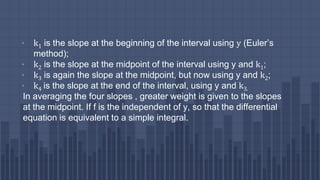
  • 9. • k1 is the slope at the beginning of the interval using y (Euler’s method); • k2 is the slope at the midpoint of the interval using y and k1; • k3 is again the slope at the midpoint, but now using y and k2; • k4 is the slope at the end of the interval, using y and k3. In averaging the four slopes , greater weight is given to the slopes at the midpoint. If f is the independent of y, so that the differential equation is equivalent to a simple integral.
  • 11. Example: Example 1: Using Runge-Kutta method Solve y’ = xy for x= 1.4. Initially x = 1, y=2 (take h= 0.2) Solution: The given differential equation is, 𝜕𝑦 𝜕𝑡 = f(x, y) = x y Given that x0 = 1, y0 = 2, and h= 0.2 First interval: K1 = h f(x0, y0) = 0.2 f(1,2) = 0.2 (1 x 2) = 0.4 11
  • 12. k2 = h f(x0 + ℎ 2 , y0 + k1 2 ) = 0.2 f(1.1 , 2.2) = 0.2 (1.1 x 2.2) = 0.484 k3 = h f(x0 + ℎ 2 , y0 + k2 2 ) = 0.2 f(1.1 , 2.242) = 0.2 (1.1 x 2.242) = 0.49324 k4 = h f(x0 + ℎ , y0 + k3) = 0.2 f(1.1 , 2.49324) = 0.2 (1.1 x 2.49324 ) = 0.5983776 x0 + ℎ 2 = 1+ 0.2 2 = 1.1 y0 + k1 2 = 2+ 0.4 2 = 2.2 y0 + k2 2 = 2 + 0.484 2 = 2.242 x0 + h =1+ 0.2 = 1.2 y0 + k3= 2 + 0.49324 = 2.49324
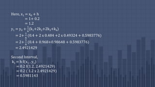
  • 13. Here, x1 = x0 + h = 1+ 0.2 = 1.2 y1 = y0 + 1 6 (k1+2k2+2k3+k4) = 2+ 1 6 (0.4 + 2 x 0.484 +2 x 0.49324 + 0.5983776) = 2+ 1 6 (0.4 + 0.968+0.98648 + 0.5983776) = 2.4921429 Second Interval, k1 = h f(x1 , y1) = 0.2 f(1.2, 2.4921429) = 0.2 ( 1.2 x 2.4921429) = 0.5981143
  • 14. k2 = h f(x1 + ℎ 2 , y1 + k1 2 ) = 0.2 f(1.3 , 2.7911999) = 0.2 (1.3 x 2.7911999) = 0.725712 k3 = h f(x1 + ℎ 2 , y1 + k2 2 ) = 0.2 f(1.3 , 2.8549989) = 0.2 (1.3 x 2.8549989) = 0.7422997 k4 = h f(x1 + ℎ , y1 + k3) = 0.2 f(1.1 , 3.2344426) = 0.2 (1.1 x 3.2344426) = 0.9056439 x1 + ℎ 2 = 1.2+ 0.2 2 = 1.3 y1 + k1 2 = 2.4921429+ 0.5981143 2 = 2.7911999 y1 + k2 2 = 2.4921429 + 0.725712 2 = 2.8549989 x1 + h =1.2+ 0.2 = 1.4 y1 + k3= 2.4921429 + 0.7422997 = 3.2344426
  • 15. Since, x2 = x1 + h = 1.2 +.2 = 1.4 and, y2 = y1 + 1 6 (k1+2k2+2k3+k4) = 2.4921429 + 1 6 ( 0.5981143 +1.451424 + 1.4845994 + 0.9056439) = 3.2321065 The value of x and y can be tabularized by: x 1 1.2 1.4 y 2 2.4921429 3.2321065
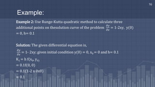
  • 16. Example: Example 2: Use Runge-Kutta quadratic method to calculate three additional points on thesolution curve of the problem 𝜕𝑦 𝜕𝑥 = 1-2xy, y(0) = 0, h= 0.1 Solution: The given differential equation is, 𝜕𝑦 𝜕𝑥 = 1- 2xy; given initial condition y(0) = 0, x0 = 0 and h= 0.1 K1 = h f(x0, y0) = 0.1f(0, 0) = 0.1(1-2 x 0x0) = 0.1 16
  • 17. k2 = h f(x0 + ℎ 2 , y0 + k1 2 ) = 0.1f(0+ 0.1 2 , 0+ 0.1 2 ) = 0.1 f(0.05 , 0.05) = 0.1 (1- 2 x0.05 x0.05) = 0.0995 k3 = h f(x0 + ℎ 2 , y0 + k2 2 ) = 0.1f(0.05, 0+ 0.0995 2 ) = 0.1 f(0.5 , 0.04975) = 0.1 (1- 2 x0.05 x 0.04975) = 0.0995025
  • 18. k4 = h f(x0 + ℎ , y0 + k3) = 0.1 f(0.1 , 0.0995025) = 0.2 (1-2x 0.1 x 0.0995025) = 0.09801 X1 = x0 + h = 0 + 0.1 = 0.1 Since, y1 = y0 + 1 6 (k1+2k2+2k3+k4) = 0 + 1 6 ( 0.1 +2x 0.0995 + 2 x 0.0995025 + 0.09801) = 1 6 ( 0.1 + 0.199 + 0.199005 + 0.09801) = 0.0993358 = 0.099336
  • 19. The value of x and y can be tabularized by: x 0 0.1 y 0 0.99336
  • 21. References: ▫ Text book: Numerical Analysis by A.R. Vasishtha and Vipin Vasishtha ▫ https://en.wikipedia.org/wiki/Runge%E2%80%93Kutta_methods ▫ https://www.quora.com/What-are-the-applications-of-the-Runge- Kutta-method-in-real-life-based 21
  • 22. Ask frequently, if you have any QUESTION???