SlideShare a Scribd company logo
Sparse Regularization
Of Inverse Problems
       Gabriel Peyré
   www.numerical-tours.com
Overview

• Inverse Problems Regularization

• Sparse Synthesis Regularization

• Examples: Sparse Wavelet Regularizations

• Iterative Soft Thresholding

• Sparse Seismic Deconvolution
Inverse Problems
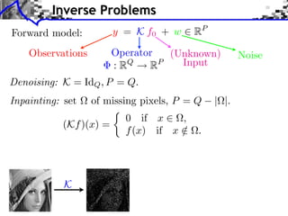
Forward model:    y = K f0 + w   RP

   Observations   Operator  (Unknown)   Noise
                  : RQ   RP   Input
Inverse Problems
Forward model:       y = K f0 + w   RP

    Observations     Operator  (Unknown)   Noise
                     : RQ   RP   Input
Denoising: K = IdQ , P = Q.
Inverse Problems
Forward model:          y = K f0 + w     RP

    Observations        Operator  (Unknown)          Noise
                        : RQ   RP   Input
Denoising: K = IdQ , P = Q.
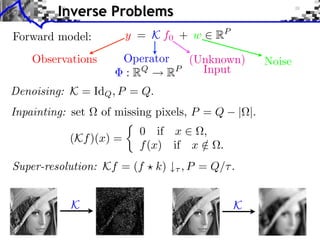
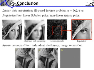
Inpainting: set    of missing pixels, P = Q   | |.
                          0 if x     ,
           (Kf )(x) =
                          f (x) if x /    .


            K
Inverse Problems
Forward model:          y = K f0 + w     RP

    Observations        Operator  (Unknown)            Noise
                        : RQ   RP   Input
Denoising: K = IdQ , P = Q.
Inpainting: set    of missing pixels, P = Q     | |.
                          0 if x     ,
           (Kf )(x) =
                          f (x) if x /    .
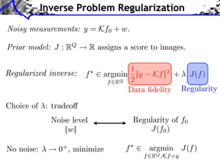
Super-resolution: Kf = (f     k)   , P = Q/ .


            K                                 K
Inverse Problem in Medical Imaging
           Kf = (p k )1   k K
Inverse Problem in Medical Imaging
                       Kf = (p k )1   k K


Magnetic resonance imaging (MRI):            ˆ
                                       Kf = (f ( ))
                                ˆ
                                f
Inverse Problem in Medical Imaging
                        Kf = (p k )1   k K


Magnetic resonance imaging (MRI):             ˆ
                                        Kf = (f ( ))
                                  ˆ
                                  f


Other examples: MEG, EEG, . . .
Inverse Problem Regularization

Noisy measurements: y = Kf0 + w.

Prior model: J : RQ   R assigns a score to images.
Inverse Problem Regularization

Noisy measurements: y = Kf0 + w.

Prior model: J : RQ   R assigns a score to images.

                                1
                      f   argmin ||y Kf ||2 + J(f )
                           f RQ 2
                                Data fidelity Regularity
Inverse Problem Regularization

Noisy measurements: y = Kf0 + w.

Prior model: J : RQ       R assigns a score to images.

                                    1
                      f       argmin ||y Kf ||2 + J(f )
                               f RQ 2
                                    Data fidelity Regularity

Choice of : tradeo
            Noise level               Regularity of f0
                ||w||                     J(f0 )
Inverse Problem Regularization

Noisy measurements: y = Kf0 + w.

Prior model: J : RQ         R assigns a score to images.

                                      1
                        f       argmin ||y Kf ||2 + J(f )
                                 f RQ 2
                                      Data fidelity Regularity

Choice of : tradeo
              Noise level                 Regularity of f0
                  ||w||                       J(f0 )

No noise:       0+ , minimize         f       argmin J(f )
                                             f RQ ,Kf =y
Smooth and Cartoon Priors

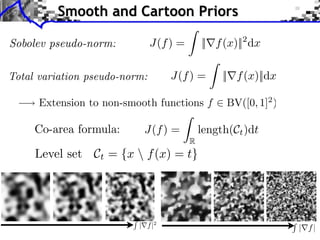
              J(f ) =   || f (x)||2 dx


           | f |2
Smooth and Cartoon Priors

              J(f ) =       || f (x)||2 dx

                    J(f ) =      || f (x)||dx


            J(f ) =         length(Ct )dt
                        R


           | f |2                               | f|
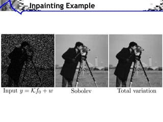
Inpainting Example


Input y = Kf0 + w   Sobolev   Total variation
Overview

• Inverse Problems Regularization

• Sparse Synthesis Regularization

• Examples: Sparse Wavelet Regularizations

• Iterative Soft Thresholding

• Sparse Seismic Deconvolution
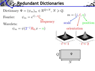
Redundant Dictionaries
Dictionary   =(   m )m   RQ   N
                                  ,N       Q.


                                       Q

                                                N
Redundant Dictionaries
Dictionary    =(    m )m        RQ   N
                                         ,N       Q.
Fourier:      m   = ei   ·, m

                                frequency


                                              Q

                                                       N
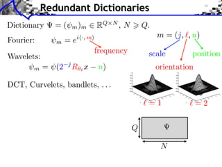
Redundant Dictionaries
Dictionary    =(       m )m      RQ    N
                                           ,N       Q.
                                                         m = (j, , n)
Fourier:      m    =e   i ·, m

                                 frequency           scale         position
Wavelets:
       m    = (2   j
                       R x        n)                     orientation


                                                     =1                =2


                                                Q

                                                          N
Redundant Dictionaries
Dictionary    =(       m )m      RQ    N
                                           ,N       Q.
                                                         m = (j, , n)
Fourier:      m    =e   i ·, m

                                 frequency           scale         position
Wavelets:
       m    = (2   j
                       R x        n)                     orientation

DCT, Curvelets, bandlets, . . .

                                                     =1                =2


                                                Q

                                                          N
Redundant Dictionaries
Dictionary    =(       m )m      RQ       N
                                              ,N       Q.
                                                            m = (j, , n)
Fourier:      m    =e   i ·, m

                                 frequency              scale         position
Wavelets:
       m    = (2   j
                       R x           n)                     orientation

DCT, Curvelets, bandlets, . . .

Synthesis: f =     m    xm       m   =    x.            =1                =2


                                                   Q                       =f
                                                                      x
                                                             N
Coe cients x       Image f =              x
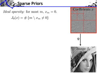
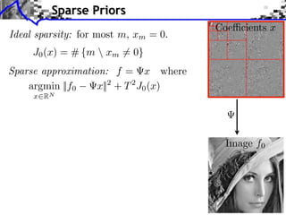
Sparse Priors
                                      Coe cients x
Ideal sparsity: for most m, xm = 0.
     J0 (x) = # {m  xm = 0}


                                        Image f0
Sparse Priors
                                       Coe cients x
Ideal sparsity: for most m, xm = 0.
     J0 (x) = # {m  xm = 0}
Sparse approximation: f = x where
    argmin ||f0    x||2 + T 2 J0 (x)
     x2RN


                                         Image f0
Sparse Priors
                                            Coe cients x
Ideal sparsity: for most m, xm = 0.
     J0 (x) = # {m  xm = 0}
Sparse approximation: f = x where
    argmin ||f0    x||2 + T 2 J0 (x)
     x2RN

Orthogonal   :      =      = IdN
       f0 , m if | f0 ,        m   | > T,
 xm =
      0 otherwise.                    ST      Image f0
   f=    ST   (f0 )

Non-orthogonal :
       NP-hard.
Convex Relaxation: L1 Prior
                       J0 (x) = # {m  xm = 0}
                        J0 (x) = 0        null image.
Image with 2 pixels:    J0 (x) = 1        sparse image.
                        J0 (x) = 2        non-sparse image.
   x2

         x1


  q=0
Convex Relaxation: L1 Prior
                             J0 (x) = # {m  xm = 0}
                               J0 (x) = 0       null image.
Image with 2 pixels:           J0 (x) = 1       sparse image.
                               J0 (x) = 2       non-sparse image.
     x2

           x1


     q=0           q = 1/2         q=1      q = 3/2       q=2
 q
     priors:        Jq (x) =       |xm |q      (convex for q    1)
                               m
Convex Relaxation: L1 Prior
                                  J0 (x) = # {m  xm = 0}
                                    J0 (x) = 0          null image.
Image with 2 pixels:                J0 (x) = 1          sparse image.
                                    J0 (x) = 2          non-sparse image.
     x2

               x1


     q=0                q = 1/2         q=1         q = 3/2       q=2
 q
     priors:             Jq (x) =       |xm |q         (convex for q    1)
                                    m


Sparse     1
               prior:      J1 (x) =         |xm |
                                        m
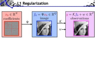
L1 Regularization

 x0 RN
coe cients
L1 Regularization

 x0 RN          f0 = x0 RQ
coe cients          image
L1 Regularization

 x0 RN          f0 = x0 RQ       y = Kf0 + w RP
coe cients          image           observations
                             K

                             w
L1 Regularization

 x0 RN          f0 = x0 RQ            y = Kf0 + w RP
coe cients          image                observations
                                  K

                              w


                 = K ⇥ ⇥ RP   N
L1 Regularization

 x0 RN            f0 = x0 RQ             y = Kf0 + w RP
coe cients            image                 observations
                                     K

                                  w


                  = K ⇥ ⇥ RP     N


 Sparse recovery: f =   x where x solves
            1
        min   ||y     x||2 + ||x||1
       x RN 2
               Fidelity Regularization
Noiseless Sparse Regularization
Noiseless measurements:        y = x0

              x
                      x=
                           y


 x    argmin          |xm |
        x=y       m
Noiseless Sparse Regularization
Noiseless measurements:        y = x0

              x
                                                 x
                      x=                              x=
                           y                               y


 x    argmin          |xm |        x    argmin       |xm |2
        x=y       m                       x=y    m
Noiseless Sparse Regularization
Noiseless measurements:          y = x0

                x
                                                        x
                        x=                                     x=
                             y                                      y


  x    argmin           |xm |          x      argmin          |xm |2
          x=y       m                            x=y     m


Convex linear program.
      Interior points, cf. [Chen, Donoho, Saunders] “basis pursuit”.
      Douglas-Rachford splitting, see [Combettes, Pesquet].
Noisy Sparse Regularization
Noisy measurements:      y = x0 + w

             1
 x    argmin ||y    x||2 + ||x||1
       x RQ 2
            Data fidelity Regularization
Noisy Sparse Regularization
Noisy measurements:      y = x0 + w

             1
 x    argmin ||y    x||2 + ||x||1
       x RQ 2                             Equivalence
            Data fidelity Regularization

 x     argmin ||x||1
      || x y||
                                          |
                                              x=
                                      x            y|
Noisy Sparse Regularization
Noisy measurements:               y = x0 + w

                 1
  x       argmin ||y    x||2 + ||x||1
           x RQ 2                                   Equivalence
                Data fidelity Regularization

  x       argmin ||x||1
         || x y||
                                                    |
                                                        x=
Algorithms:                                     x            y|
      Iterative soft thresholding
             Forward-backward splitting
 see [Daubechies et al], [Pesquet et al], etc
      Nesterov multi-steps schemes.
Overview

• Inverse Problems Regularization

• Sparse Synthesis Regularization

• Examples: Sparse Wavelet Regularizations

• Iterative Soft Thresholding

• Sparse Seismic Deconvolution
Image De-blurring


Original f0   y = h f0 + w
Image De-blurring


  Original f0     y = h f0 + w           Sobolev
                                       SNR=22.7dB
Sobolev regularization:   f = argmin ||f ⇥ h   y||2 + ||⇥f ||2
                                 f RN
                          ˆ
                          h(⇥)
          ˆ
          f (⇥) =                    y (⇥)
                                     ˆ
                     ˆ
                    |h(⇥)|2 + |⇥|2
Image De-blurring


  Original f0      y = h f0 + w            Sobolev            Sparsity
                                         SNR=22.7dB        SNR=24.7dB
Sobolev regularization:       f = argmin ||f ⇥ h   y||2 + ||⇥f ||2
                                     f RN
                              ˆ
                              h(⇥)
            ˆ
            f (⇥) =                    y (⇥)
                                       ˆ
                       ˆ
                      |h(⇥)|2 + |⇥|2

Sparsity regularization:          = translation invariant wavelets.
                                        1
f =     x       where     x      argmin ||h ( x) y||2 + ||x||1
                                    x   2
Comparison of Regularizations
  L2 regularization      Sobolev regularization   Sparsity regularization
SNR


                          SNR


                                                   SNR
      opt                            opt                 opt


   L2                   Sobolev         Sparsity           Invariant
SNR=21.7dB            SNR=22.7dB      SNR=23.7dB          SNR=24.7dB
Inpainting Problem


               K                         0 if x     ,
                            (Kf )(x) =
                                         f (x) if x /   .

Measures:     y = Kf0 + w
Image Separation
Model: f = f1 + f2 + w, (f1 , f2 ) components, w noise.
Image Separation
Model: f = f1 + f2 + w, (f1 , f2 ) components, w noise.
Image Separation
Model: f = f1 + f2 + w, (f1 , f2 ) components, w noise.


Union dictionary:         =[    1,     2]      RQ   (N1 +N2 )


Recovered component: fi =            i xi .
                                       1
         (x1 , x2 )      argmin          ||f        x||2 + ||x||1
                      x=(x1 ,x2 ) RN   2
Examples of Decompositions
Cartoon+Texture Separation
Overview

• Inverse Problems Regularization

• Sparse Synthesis Regularization

• Examples: Sparse Wavelet Regularizations

• Iterative Soft Thresholding

• Sparse Seismic Deconvolution
Sparse Regularization Denoising
Denoising: y = x0 + w 2 RN , K = Id.
                     ⇤                 ⇤
Orthogonal-basis:        = IdN , x =       f.
Regularization-based denoising:
                           1
              x = argmin ||x y||2 + J(x)
                ?
                     x2RN 2
                             P
Sparse regularization: J(x) = m |xm |q
       (where |a|0 = (a))
Sparse Regularization Denoising
Denoising: y = x0 + w 2 RN , K = Id.
                        ⇤                 ⇤
Orthogonal-basis:           = IdN , x =       f.
Regularization-based denoising:
                           1
              x = argmin ||x y||2 + J(x)
                ?
                     x2RN 2
                             P
Sparse regularization: J(x) = m |xm |q
       (where |a|0 = (a))

                     q
           x?
            m   =   ST (xm )
Surrogate Functionals
Sparse regularization:
            ?               1
           x 2 argmin E(x) = ||y               x||2 + ||x||1
                 x2RN       2
                                      ⇤
Surrogate functional:      ⌧ < 1/||       ||
                        1             2  1
 E(x, x) = E(x)
      ˜                   || (x   x)|| + ||x
                                  ˜                   x||2
                                                      ˜
                        2               2⌧
                                                       E(·, x)
                                                            ˜

                                               E(·)

                                                                         x
                                                             S ⌧ (u) x
                                                                     ˜
Surrogate Functionals
Sparse regularization:
            ?               1
           x 2 argmin E(x) = ||y                 x||2 + ||x||1
                 x2RN       2
                                        ⇤
Surrogate functional:       ⌧ < 1/||        ||
                        1               2    1
 E(x, x) = E(x)
      ˜                   || (x       x)|| + ||x
                                      ˜                 x||2
                                                        ˜
                        2                   2⌧
                                                         E(·, x)
                                                              ˜
   Theorem:
     argmin E(x, x) = S ⌧ (u)
                 ˜                               E(·)
          x
                            ⇤
    where u = x         ⌧       ( x    x)
                                       ˜
                                                                           x
                                                               S ⌧ (u) x
                                                                       ˜

 Proof: E(x, x) / 1 ||u
             ˜    2             x||2 + ||x||1 + cst.
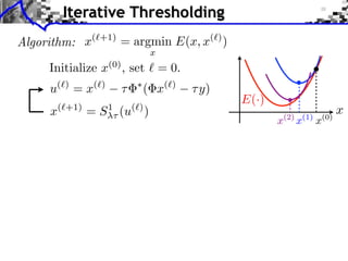
Iterative Thresholding
Algorithm: x(`+1) = argmin E(x, x(`) )
                             x
     Initialize x(0) , set ` = 0.
                        ⇤
     u(`) = x(`)    ⌧       ( x(`)   ⌧ y)
                                            E(·)
     x(`+1) = S 1⌧ (u(`) )                             (2)       (1)       (0)
                                                                                 x
                                                   x         x         x
Iterative Thresholding
Algorithm: x(`+1) = argmin E(x, x(`) )
                              x
     Initialize x(0) , set ` = 0.
                         ⇤
     u(`) = x(`)     ⌧       ( x(`)   ⌧ y)
                                             E(·)
      x(`+1) = S 1⌧ (u(`) )                             (2)       (1)       (0)
                                                                                  x
                                                    x         x         x
Remark:
    x(`) 7! u(`) is a gradient descent of || x y||2 .
     1
    S`⌧ is the proximal step of associated to ||x||1 .
Iterative Thresholding
Algorithm: x(`+1) = argmin E(x, x(`) )
                              x
     Initialize x(0) , set ` = 0.
                         ⇤
     u(`) = x(`)     ⌧       ( x(`)    ⌧ y)
                                                 E(·)
      x(`+1) = S 1⌧ (u(`) )                                  (2)       (1)       (0)
                                                                                       x
                                                        x          x         x
Remark:
    x(`) 7! u(`) is a gradient descent of || x y||2 .
     1
    S`⌧ is the proximal step of associated to ||x||1 .


                                  ⇤
      Theorem: if ⌧ < 2/||            ||, then x(`) ! x? .
Overview

• Inverse Problems Regularization

• Sparse Synthesis Regularization

• Examples: Sparse Wavelet Regularizations

• Iterative Soft Thresholding

• Sparse Seismic Deconvolution
Seismic Imaging
1D Idealization
               Initial condition: “wavelet”
                      = band pass filter h

                   1D propagation convolution
                           f =h f

                                              h(x)

               f

                                              ˆ
                                              h( )


y = f0 h + w                      P
Pseudo Inverse
Pseudo-inverse:

   ˆ+ ( ) = y ( )
   f
            ˆ
                    =      f + = h+ ⇥ y = f0 + h+ ⇥ w
            h( )
                                     ˆ        ˆ
                               where h+ ( ) = h( )   1


               ˆ              ˆ
Stabilization: h+ (⇥) = 0 if |h(⇥)|

                        ˆ
                        h( )                   y = h f0 + w


                      ˆ
                    1/h( )

                                                         f+
Sparse Spikes Deconvolution


    f with small ||f ||0                 y=f        h+w
Sparsity basis: Diracs     ⇥m [x] = [x   m]
                       1
             f = argmin ||f ⇥ h    y||2 +         |f [m]|.
                  f RN 2                      m
Sparse Spikes Deconvolution


    f with small ||f ||0                     y=f        h+w
Sparsity basis: Diracs      ⇥m [x] = [x      m]
                       1
             f = argmin ||f ⇥ h        y||2 +         |f [m]|.
                  f RN 2                          m


Algorithm:         < 2/||                 ˆ
                              || = 2/max |h(⇥)|2
                   ˜
      • Inversion: f (k) = f (k)     h ⇥ (h ⇥ f (k)    y).
                                         ˜
                     f (k+1) [m] = S 1⇥ (f (k) [m])
Numerical Example

                                        f0
Choosing optimal :
 oracle, minimize ||f0   f ||

                                y=f   h+w
SNR(f0 , f )


                                       f
Convergence Study
Sparse deconvolution:f = argmin E(f ).
                            f RN
                    1
     Energy: E(f ) = ||h ⇥ f y||2 +    |f [m]|.
                    2               m
Not strictly convex      =    no convergence speed.

log10 (E(f (k) )/E(f )   1)        log10 (||f (k)   f ||/||f0 ||)


                              k                                     k
Conclusion
Conclusion
Conclusion

More Related Content

What's hot (20)

PPTX
マルコフ連鎖モンテカルロ法と多重代入法
Koichiro Gibo
 
PPTX
ImageJを使った画像解析実習〜大量の画像データに対する処理の自動化〜
LPIXEL
 
PDF
アンサンブル木モデル解釈のためのモデル簡略化法
Satoshi Hara
 
PDF
機械学習のためのベイズ最適化入門
hoxo_m
 
PPT
「診断精度研究のメタ分析」の入門
yokomitsuken5
 
PDF
バリデーション研究の入門
Yasuyuki Okumura
 
PDF
[第2版]Python機械学習プログラミング 第6章
Haruki Eguchi
 
PPTX
[DL輪読会]Swin Transformer: Hierarchical Vision Transformer using Shifted Windows
Deep Learning JP
 
PDF
ガイデットフィルタとその周辺
Norishige Fukushima
 
PPTX
【DL輪読会】マルチモーダル 基盤モデル
Deep Learning JP
 
PDF
シンギュラリティを知らずに機械学習を語るな
hoxo_m
 
PDF
臨床疫学研究における傾向スコア分析の使い⽅ 〜観察研究における治療効果研究〜
Yasuyuki Okumura
 
PPTX
Semi supervised, weakly-supervised, unsupervised, and active learning
Yusuke Uchida
 
PPTX
遠赤外線カメラと可視カメラを利用した悪条件下における画像取得
Masayuki Tanaka
 
PPTX
Optimisation par colonie de fourmis par zellagui amine
Zellagui Amine
 
PPTX
2016.9.24診断精度の系統的レビューワークショップ事前課題 "質の評価とアウトカム"
SR WS
 
PDF
[DL輪読会]SlowFast Networks for Video Recognition
Deep Learning JP
 
PDF
計量経済学と 機械学習の交差点入り口 (公開用)
Shota Yasui
 
PDF
【DL輪読会】“Gestalt Principles Emerge When Learning Universal Sound Source Separa...
Deep Learning JP
 
PPTX
【DL輪読会】Responsive Safety in Reinforcement Learning by PID Lagrangian Methods...
Deep Learning JP
 
マルコフ連鎖モンテカルロ法と多重代入法
Koichiro Gibo
 
ImageJを使った画像解析実習〜大量の画像データに対する処理の自動化〜
LPIXEL
 
アンサンブル木モデル解釈のためのモデル簡略化法
Satoshi Hara
 
機械学習のためのベイズ最適化入門
hoxo_m
 
「診断精度研究のメタ分析」の入門
yokomitsuken5
 
バリデーション研究の入門
Yasuyuki Okumura
 
[第2版]Python機械学習プログラミング 第6章
Haruki Eguchi
 
[DL輪読会]Swin Transformer: Hierarchical Vision Transformer using Shifted Windows
Deep Learning JP
 
ガイデットフィルタとその周辺
Norishige Fukushima
 
【DL輪読会】マルチモーダル 基盤モデル
Deep Learning JP
 
シンギュラリティを知らずに機械学習を語るな
hoxo_m
 
臨床疫学研究における傾向スコア分析の使い⽅ 〜観察研究における治療効果研究〜
Yasuyuki Okumura
 
Semi supervised, weakly-supervised, unsupervised, and active learning
Yusuke Uchida
 
遠赤外線カメラと可視カメラを利用した悪条件下における画像取得
Masayuki Tanaka
 
Optimisation par colonie de fourmis par zellagui amine
Zellagui Amine
 
2016.9.24診断精度の系統的レビューワークショップ事前課題 "質の評価とアウトカム"
SR WS
 
[DL輪読会]SlowFast Networks for Video Recognition
Deep Learning JP
 
計量経済学と 機械学習の交差点入り口 (公開用)
Shota Yasui
 
【DL輪読会】“Gestalt Principles Emerge When Learning Universal Sound Source Separa...
Deep Learning JP
 
【DL輪読会】Responsive Safety in Reinforcement Learning by PID Lagrangian Methods...
Deep Learning JP
 

Viewers also liked (9)

PDF
Signal Processing Course : Convex Optimization
Gabriel Peyré
 
PDF
Signal Processing Course : Approximation
Gabriel Peyré
 
PDF
Signal Processing Course : Inverse Problems Regularization
Gabriel Peyré
 
PDF
Digital Signal Processing - Practical Techniques, Tips and Tricks Course Sampler
Jim Jenkins
 
PDF
C2.5
Daniel LIAO
 
PDF
Signal Processing Course : Theory for Sparse Recovery
Gabriel Peyré
 
PDF
Signal Processing Course : Compressed Sensing
Gabriel Peyré
 
PDF
Energy proposition
Ewan Rawlings
 
Signal Processing Course : Convex Optimization
Gabriel Peyré
 
Signal Processing Course : Approximation
Gabriel Peyré
 
Signal Processing Course : Inverse Problems Regularization
Gabriel Peyré
 
Digital Signal Processing - Practical Techniques, Tips and Tricks Course Sampler
Jim Jenkins
 
Signal Processing Course : Theory for Sparse Recovery
Gabriel Peyré
 
Signal Processing Course : Compressed Sensing
Gabriel Peyré
 
Energy proposition
Ewan Rawlings
 
Ad

Similar to Signal Processing Course : Sparse Regularization of Inverse Problems (20)

PDF
Sparsity and Compressed Sensing
Gabriel Peyré
 
PDF
Adaptive Signal and Image Processing
Gabriel Peyré
 
PDF
A Review of Proximal Methods, with a New One
Gabriel Peyré
 
PDF
Compressed Sensing and Tomography
Gabriel Peyré
 
PDF
quantization
aniruddh Tyagi
 
PDF
quantization
aniruddh Tyagi
 
PDF
quantization
Aniruddh Tyagi
 
PDF
Tall-and-skinny QR factorizations in MapReduce architectures
David Gleich
 
PDF
A hand-waving introduction to sparsity for compressed tomography reconstruction
Gael Varoquaux
 
PDF
Learning Sparse Representation
Gabriel Peyré
 
PDF
omp-and-k-svd - Gdc2013
Manchor Ko
 
PDF
Tro07 sparse-solutions-talk
mpbchina
 
PDF
Low Complexity Regularization of Inverse Problems - Course #1 Inverse Problems
Gabriel Peyré
 
PPTX
imagetransforms1-210417050321.pptx
MrsSDivyaBME
 
PDF
Direct tall-and-skinny QR factorizations in MapReduce architectures
David Gleich
 
PDF
Tuto part2
Bo Li
 
PDF
Robust Super-Resolution by minimizing a Gaussian-weighted L2 error norm
Tuan Q. Pham
 
PDF
DIGITAL IMAGE PROCESSING - Day 4 Image Transform
vijayanand Kandaswamy
 
PDF
Signal Processing Course : Orthogonal Bases
Gabriel Peyré
 
Sparsity and Compressed Sensing
Gabriel Peyré
 
Adaptive Signal and Image Processing
Gabriel Peyré
 
A Review of Proximal Methods, with a New One
Gabriel Peyré
 
Compressed Sensing and Tomography
Gabriel Peyré
 
quantization
aniruddh Tyagi
 
quantization
aniruddh Tyagi
 
quantization
Aniruddh Tyagi
 
Tall-and-skinny QR factorizations in MapReduce architectures
David Gleich
 
A hand-waving introduction to sparsity for compressed tomography reconstruction
Gael Varoquaux
 
Learning Sparse Representation
Gabriel Peyré
 
omp-and-k-svd - Gdc2013
Manchor Ko
 
Tro07 sparse-solutions-talk
mpbchina
 
Low Complexity Regularization of Inverse Problems - Course #1 Inverse Problems
Gabriel Peyré
 
imagetransforms1-210417050321.pptx
MrsSDivyaBME
 
Direct tall-and-skinny QR factorizations in MapReduce architectures
David Gleich
 
Tuto part2
Bo Li
 
Robust Super-Resolution by minimizing a Gaussian-weighted L2 error norm
Tuan Q. Pham
 
DIGITAL IMAGE PROCESSING - Day 4 Image Transform
vijayanand Kandaswamy
 
Signal Processing Course : Orthogonal Bases
Gabriel Peyré
 
Ad

More from Gabriel Peyré (19)

PDF
Low Complexity Regularization of Inverse Problems - Course #3 Proximal Splitt...
Gabriel Peyré
 
PDF
Low Complexity Regularization of Inverse Problems - Course #2 Recovery Guaran...
Gabriel Peyré
 
PDF
Low Complexity Regularization of Inverse Problems
Gabriel Peyré
 
PDF
Model Selection with Piecewise Regular Gauges
Gabriel Peyré
 
PDF
Proximal Splitting and Optimal Transport
Gabriel Peyré
 
PDF
Geodesic Method in Computer Vision and Graphics
Gabriel Peyré
 
PDF
Mesh Processing Course : Mesh Parameterization
Gabriel Peyré
 
PDF
Mesh Processing Course : Multiresolution
Gabriel Peyré
 
PDF
Mesh Processing Course : Introduction
Gabriel Peyré
 
PDF
Mesh Processing Course : Geodesics
Gabriel Peyré
 
PDF
Mesh Processing Course : Geodesic Sampling
Gabriel Peyré
 
PDF
Mesh Processing Course : Differential Calculus
Gabriel Peyré
 
PDF
Mesh Processing Course : Active Contours
Gabriel Peyré
 
PDF
Signal Processing Course : Presentation of the Course
Gabriel Peyré
 
PDF
Signal Processing Course : Fourier
Gabriel Peyré
 
PDF
Signal Processing Course : Denoising
Gabriel Peyré
 
PDF
Signal Processing Course : Wavelets
Gabriel Peyré
 
PDF
Optimal Transport in Imaging Sciences
Gabriel Peyré
 
PDF
An Introduction to Optimal Transport
Gabriel Peyré
 
Low Complexity Regularization of Inverse Problems - Course #3 Proximal Splitt...
Gabriel Peyré
 
Low Complexity Regularization of Inverse Problems - Course #2 Recovery Guaran...
Gabriel Peyré
 
Low Complexity Regularization of Inverse Problems
Gabriel Peyré
 
Model Selection with Piecewise Regular Gauges
Gabriel Peyré
 
Proximal Splitting and Optimal Transport
Gabriel Peyré
 
Geodesic Method in Computer Vision and Graphics
Gabriel Peyré
 
Mesh Processing Course : Mesh Parameterization
Gabriel Peyré
 
Mesh Processing Course : Multiresolution
Gabriel Peyré
 
Mesh Processing Course : Introduction
Gabriel Peyré
 
Mesh Processing Course : Geodesics
Gabriel Peyré
 
Mesh Processing Course : Geodesic Sampling
Gabriel Peyré
 
Mesh Processing Course : Differential Calculus
Gabriel Peyré
 
Mesh Processing Course : Active Contours
Gabriel Peyré
 
Signal Processing Course : Presentation of the Course
Gabriel Peyré
 
Signal Processing Course : Fourier
Gabriel Peyré
 
Signal Processing Course : Denoising
Gabriel Peyré
 
Signal Processing Course : Wavelets
Gabriel Peyré
 
Optimal Transport in Imaging Sciences
Gabriel Peyré
 
An Introduction to Optimal Transport
Gabriel Peyré
 

Signal Processing Course : Sparse Regularization of Inverse Problems

  • 1. Sparse Regularization Of Inverse Problems Gabriel Peyré www.numerical-tours.com
  • 2. Overview • Inverse Problems Regularization • Sparse Synthesis Regularization • Examples: Sparse Wavelet Regularizations • Iterative Soft Thresholding • Sparse Seismic Deconvolution
  • 3. Inverse Problems Forward model: y = K f0 + w RP Observations Operator (Unknown) Noise : RQ RP Input
  • 4. Inverse Problems Forward model: y = K f0 + w RP Observations Operator (Unknown) Noise : RQ RP Input Denoising: K = IdQ , P = Q.
  • 5. Inverse Problems Forward model: y = K f0 + w RP Observations Operator (Unknown) Noise : RQ RP Input Denoising: K = IdQ , P = Q. Inpainting: set of missing pixels, P = Q | |. 0 if x , (Kf )(x) = f (x) if x / . K
  • 6. Inverse Problems Forward model: y = K f0 + w RP Observations Operator (Unknown) Noise : RQ RP Input Denoising: K = IdQ , P = Q. Inpainting: set of missing pixels, P = Q | |. 0 if x , (Kf )(x) = f (x) if x / . Super-resolution: Kf = (f k) , P = Q/ . K K
  • 7. Inverse Problem in Medical Imaging Kf = (p k )1 k K
  • 8. Inverse Problem in Medical Imaging Kf = (p k )1 k K Magnetic resonance imaging (MRI): ˆ Kf = (f ( )) ˆ f
  • 9. Inverse Problem in Medical Imaging Kf = (p k )1 k K Magnetic resonance imaging (MRI): ˆ Kf = (f ( )) ˆ f Other examples: MEG, EEG, . . .
  • 10. Inverse Problem Regularization Noisy measurements: y = Kf0 + w. Prior model: J : RQ R assigns a score to images.
  • 11. Inverse Problem Regularization Noisy measurements: y = Kf0 + w. Prior model: J : RQ R assigns a score to images. 1 f argmin ||y Kf ||2 + J(f ) f RQ 2 Data fidelity Regularity
  • 12. Inverse Problem Regularization Noisy measurements: y = Kf0 + w. Prior model: J : RQ R assigns a score to images. 1 f argmin ||y Kf ||2 + J(f ) f RQ 2 Data fidelity Regularity Choice of : tradeo Noise level Regularity of f0 ||w|| J(f0 )
  • 13. Inverse Problem Regularization Noisy measurements: y = Kf0 + w. Prior model: J : RQ R assigns a score to images. 1 f argmin ||y Kf ||2 + J(f ) f RQ 2 Data fidelity Regularity Choice of : tradeo Noise level Regularity of f0 ||w|| J(f0 ) No noise: 0+ , minimize f argmin J(f ) f RQ ,Kf =y
  • 14. Smooth and Cartoon Priors J(f ) = || f (x)||2 dx | f |2
  • 15. Smooth and Cartoon Priors J(f ) = || f (x)||2 dx J(f ) = || f (x)||dx J(f ) = length(Ct )dt R | f |2 | f|
  • 16. Inpainting Example Input y = Kf0 + w Sobolev Total variation
  • 17. Overview • Inverse Problems Regularization • Sparse Synthesis Regularization • Examples: Sparse Wavelet Regularizations • Iterative Soft Thresholding • Sparse Seismic Deconvolution
  • 18. Redundant Dictionaries Dictionary =( m )m RQ N ,N Q. Q N
  • 19. Redundant Dictionaries Dictionary =( m )m RQ N ,N Q. Fourier: m = ei ·, m frequency Q N
  • 20. Redundant Dictionaries Dictionary =( m )m RQ N ,N Q. m = (j, , n) Fourier: m =e i ·, m frequency scale position Wavelets: m = (2 j R x n) orientation =1 =2 Q N
  • 21. Redundant Dictionaries Dictionary =( m )m RQ N ,N Q. m = (j, , n) Fourier: m =e i ·, m frequency scale position Wavelets: m = (2 j R x n) orientation DCT, Curvelets, bandlets, . . . =1 =2 Q N
  • 22. Redundant Dictionaries Dictionary =( m )m RQ N ,N Q. m = (j, , n) Fourier: m =e i ·, m frequency scale position Wavelets: m = (2 j R x n) orientation DCT, Curvelets, bandlets, . . . Synthesis: f = m xm m = x. =1 =2 Q =f x N Coe cients x Image f = x
  • 23. Sparse Priors Coe cients x Ideal sparsity: for most m, xm = 0. J0 (x) = # {m xm = 0} Image f0
  • 24. Sparse Priors Coe cients x Ideal sparsity: for most m, xm = 0. J0 (x) = # {m xm = 0} Sparse approximation: f = x where argmin ||f0 x||2 + T 2 J0 (x) x2RN Image f0
  • 25. Sparse Priors Coe cients x Ideal sparsity: for most m, xm = 0. J0 (x) = # {m xm = 0} Sparse approximation: f = x where argmin ||f0 x||2 + T 2 J0 (x) x2RN Orthogonal : = = IdN f0 , m if | f0 , m | > T, xm = 0 otherwise. ST Image f0 f= ST (f0 )
  • 26. Sparse Priors Coe cients x Ideal sparsity: for most m, xm = 0. J0 (x) = # {m xm = 0} Sparse approximation: f = x where argmin ||f0 x||2 + T 2 J0 (x) x2RN Orthogonal : = = IdN f0 , m if | f0 , m | > T, xm = 0 otherwise. ST Image f0 f= ST (f0 ) Non-orthogonal : NP-hard.
  • 27. Convex Relaxation: L1 Prior J0 (x) = # {m xm = 0} J0 (x) = 0 null image. Image with 2 pixels: J0 (x) = 1 sparse image. J0 (x) = 2 non-sparse image. x2 x1 q=0
  • 28. Convex Relaxation: L1 Prior J0 (x) = # {m xm = 0} J0 (x) = 0 null image. Image with 2 pixels: J0 (x) = 1 sparse image. J0 (x) = 2 non-sparse image. x2 x1 q=0 q = 1/2 q=1 q = 3/2 q=2 q priors: Jq (x) = |xm |q (convex for q 1) m
  • 29. Convex Relaxation: L1 Prior J0 (x) = # {m xm = 0} J0 (x) = 0 null image. Image with 2 pixels: J0 (x) = 1 sparse image. J0 (x) = 2 non-sparse image. x2 x1 q=0 q = 1/2 q=1 q = 3/2 q=2 q priors: Jq (x) = |xm |q (convex for q 1) m Sparse 1 prior: J1 (x) = |xm | m
  • 30. L1 Regularization x0 RN coe cients
  • 31. L1 Regularization x0 RN f0 = x0 RQ coe cients image
  • 32. L1 Regularization x0 RN f0 = x0 RQ y = Kf0 + w RP coe cients image observations K w
  • 33. L1 Regularization x0 RN f0 = x0 RQ y = Kf0 + w RP coe cients image observations K w = K ⇥ ⇥ RP N
  • 34. L1 Regularization x0 RN f0 = x0 RQ y = Kf0 + w RP coe cients image observations K w = K ⇥ ⇥ RP N Sparse recovery: f = x where x solves 1 min ||y x||2 + ||x||1 x RN 2 Fidelity Regularization
  • 35. Noiseless Sparse Regularization Noiseless measurements: y = x0 x x= y x argmin |xm | x=y m
  • 36. Noiseless Sparse Regularization Noiseless measurements: y = x0 x x x= x= y y x argmin |xm | x argmin |xm |2 x=y m x=y m
  • 37. Noiseless Sparse Regularization Noiseless measurements: y = x0 x x x= x= y y x argmin |xm | x argmin |xm |2 x=y m x=y m Convex linear program. Interior points, cf. [Chen, Donoho, Saunders] “basis pursuit”. Douglas-Rachford splitting, see [Combettes, Pesquet].
  • 38. Noisy Sparse Regularization Noisy measurements: y = x0 + w 1 x argmin ||y x||2 + ||x||1 x RQ 2 Data fidelity Regularization
  • 39. Noisy Sparse Regularization Noisy measurements: y = x0 + w 1 x argmin ||y x||2 + ||x||1 x RQ 2 Equivalence Data fidelity Regularization x argmin ||x||1 || x y|| | x= x y|
  • 40. Noisy Sparse Regularization Noisy measurements: y = x0 + w 1 x argmin ||y x||2 + ||x||1 x RQ 2 Equivalence Data fidelity Regularization x argmin ||x||1 || x y|| | x= Algorithms: x y| Iterative soft thresholding Forward-backward splitting see [Daubechies et al], [Pesquet et al], etc Nesterov multi-steps schemes.
  • 41. Overview • Inverse Problems Regularization • Sparse Synthesis Regularization • Examples: Sparse Wavelet Regularizations • Iterative Soft Thresholding • Sparse Seismic Deconvolution
  • 43. Image De-blurring Original f0 y = h f0 + w Sobolev SNR=22.7dB Sobolev regularization: f = argmin ||f ⇥ h y||2 + ||⇥f ||2 f RN ˆ h(⇥) ˆ f (⇥) = y (⇥) ˆ ˆ |h(⇥)|2 + |⇥|2
  • 44. Image De-blurring Original f0 y = h f0 + w Sobolev Sparsity SNR=22.7dB SNR=24.7dB Sobolev regularization: f = argmin ||f ⇥ h y||2 + ||⇥f ||2 f RN ˆ h(⇥) ˆ f (⇥) = y (⇥) ˆ ˆ |h(⇥)|2 + |⇥|2 Sparsity regularization: = translation invariant wavelets. 1 f = x where x argmin ||h ( x) y||2 + ||x||1 x 2
  • 45. Comparison of Regularizations L2 regularization Sobolev regularization Sparsity regularization SNR SNR SNR opt opt opt L2 Sobolev Sparsity Invariant SNR=21.7dB SNR=22.7dB SNR=23.7dB SNR=24.7dB
  • 46. Inpainting Problem K 0 if x , (Kf )(x) = f (x) if x / . Measures: y = Kf0 + w
  • 47. Image Separation Model: f = f1 + f2 + w, (f1 , f2 ) components, w noise.
  • 48. Image Separation Model: f = f1 + f2 + w, (f1 , f2 ) components, w noise.
  • 49. Image Separation Model: f = f1 + f2 + w, (f1 , f2 ) components, w noise. Union dictionary: =[ 1, 2] RQ (N1 +N2 ) Recovered component: fi = i xi . 1 (x1 , x2 ) argmin ||f x||2 + ||x||1 x=(x1 ,x2 ) RN 2
  • 52. Overview • Inverse Problems Regularization • Sparse Synthesis Regularization • Examples: Sparse Wavelet Regularizations • Iterative Soft Thresholding • Sparse Seismic Deconvolution
  • 53. Sparse Regularization Denoising Denoising: y = x0 + w 2 RN , K = Id. ⇤ ⇤ Orthogonal-basis: = IdN , x = f. Regularization-based denoising: 1 x = argmin ||x y||2 + J(x) ? x2RN 2 P Sparse regularization: J(x) = m |xm |q (where |a|0 = (a))
  • 54. Sparse Regularization Denoising Denoising: y = x0 + w 2 RN , K = Id. ⇤ ⇤ Orthogonal-basis: = IdN , x = f. Regularization-based denoising: 1 x = argmin ||x y||2 + J(x) ? x2RN 2 P Sparse regularization: J(x) = m |xm |q (where |a|0 = (a)) q x? m = ST (xm )
  • 55. Surrogate Functionals Sparse regularization: ? 1 x 2 argmin E(x) = ||y x||2 + ||x||1 x2RN 2 ⇤ Surrogate functional: ⌧ < 1/|| || 1 2 1 E(x, x) = E(x) ˜ || (x x)|| + ||x ˜ x||2 ˜ 2 2⌧ E(·, x) ˜ E(·) x S ⌧ (u) x ˜
  • 56. Surrogate Functionals Sparse regularization: ? 1 x 2 argmin E(x) = ||y x||2 + ||x||1 x2RN 2 ⇤ Surrogate functional: ⌧ < 1/|| || 1 2 1 E(x, x) = E(x) ˜ || (x x)|| + ||x ˜ x||2 ˜ 2 2⌧ E(·, x) ˜ Theorem: argmin E(x, x) = S ⌧ (u) ˜ E(·) x ⇤ where u = x ⌧ ( x x) ˜ x S ⌧ (u) x ˜ Proof: E(x, x) / 1 ||u ˜ 2 x||2 + ||x||1 + cst.
  • 57. Iterative Thresholding Algorithm: x(`+1) = argmin E(x, x(`) ) x Initialize x(0) , set ` = 0. ⇤ u(`) = x(`) ⌧ ( x(`) ⌧ y) E(·) x(`+1) = S 1⌧ (u(`) ) (2) (1) (0) x x x x
  • 58. Iterative Thresholding Algorithm: x(`+1) = argmin E(x, x(`) ) x Initialize x(0) , set ` = 0. ⇤ u(`) = x(`) ⌧ ( x(`) ⌧ y) E(·) x(`+1) = S 1⌧ (u(`) ) (2) (1) (0) x x x x Remark: x(`) 7! u(`) is a gradient descent of || x y||2 . 1 S`⌧ is the proximal step of associated to ||x||1 .
  • 59. Iterative Thresholding Algorithm: x(`+1) = argmin E(x, x(`) ) x Initialize x(0) , set ` = 0. ⇤ u(`) = x(`) ⌧ ( x(`) ⌧ y) E(·) x(`+1) = S 1⌧ (u(`) ) (2) (1) (0) x x x x Remark: x(`) 7! u(`) is a gradient descent of || x y||2 . 1 S`⌧ is the proximal step of associated to ||x||1 . ⇤ Theorem: if ⌧ < 2/|| ||, then x(`) ! x? .
  • 60. Overview • Inverse Problems Regularization • Sparse Synthesis Regularization • Examples: Sparse Wavelet Regularizations • Iterative Soft Thresholding • Sparse Seismic Deconvolution
  • 62. 1D Idealization Initial condition: “wavelet” = band pass filter h 1D propagation convolution f =h f h(x) f ˆ h( ) y = f0 h + w P
  • 63. Pseudo Inverse Pseudo-inverse: ˆ+ ( ) = y ( ) f ˆ = f + = h+ ⇥ y = f0 + h+ ⇥ w h( ) ˆ ˆ where h+ ( ) = h( ) 1 ˆ ˆ Stabilization: h+ (⇥) = 0 if |h(⇥)| ˆ h( ) y = h f0 + w ˆ 1/h( ) f+
  • 64. Sparse Spikes Deconvolution f with small ||f ||0 y=f h+w Sparsity basis: Diracs ⇥m [x] = [x m] 1 f = argmin ||f ⇥ h y||2 + |f [m]|. f RN 2 m
  • 65. Sparse Spikes Deconvolution f with small ||f ||0 y=f h+w Sparsity basis: Diracs ⇥m [x] = [x m] 1 f = argmin ||f ⇥ h y||2 + |f [m]|. f RN 2 m Algorithm: < 2/|| ˆ || = 2/max |h(⇥)|2 ˜ • Inversion: f (k) = f (k) h ⇥ (h ⇥ f (k) y). ˜ f (k+1) [m] = S 1⇥ (f (k) [m])
  • 66. Numerical Example f0 Choosing optimal : oracle, minimize ||f0 f || y=f h+w SNR(f0 , f ) f
  • 67. Convergence Study Sparse deconvolution:f = argmin E(f ). f RN 1 Energy: E(f ) = ||h ⇥ f y||2 + |f [m]|. 2 m Not strictly convex = no convergence speed. log10 (E(f (k) )/E(f ) 1) log10 (||f (k) f ||/||f0 ||) k k