Sorting algos > Data Structures & Algorithums
Download as PPT, PDF1 like694 views

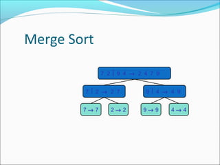
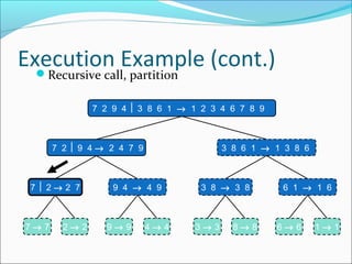
The document describes the merge sort algorithm. Merge sort is a sorting algorithm that works by dividing an unsorted list into halves, recursively sorting each half, and then merging the sorted halves into one sorted list. It has the following steps: 1. Divide: Partition the input list into equal halves. 2. Conquer: Recursively sort each half by repeating steps 1 and 2. 3. Combine: Merge the sorted halves into one sorted output list. The algorithm has a runtime of O(n log n), making it an efficient sorting algorithm for large data sets. An example execution is shown step-by-step to demonstrate how merge sort partitions, recursively sorts, and merges sublists to produce


![Static Method mergeSort()
Public static void mergeSort(a, int left, int right)
{
// sort a[left:right]
if (left < right)
{// at least two elements
int mid = (left+right)/2;
//midpoint
mergeSort(a, left, mid);
mergeSort(a, mid + 1, right);
merge(a, b, left, mid, right); //merge from a to b
copy(b, a, left, right); //copy result back to a
}
}](https://image.slidesharecdn.com/sortingalgos-140215040112-phpapp02/85/Sorting-algos-Data-Structures-Algorithums-15-320.jpg)


![Quicksort - Partition
int partition( int *a, int low, int high ) {
int left, right;
int pivot_item;
pivot_item = a[low];
pivot = left = low;
right = high;
while ( left < right ) {
/* Move left while item < pivot */
while( a[left] <= pivot_item ) left++;
/* Move right while item > pivot */
while( a[right] >= pivot_item ) right--;
if ( left < right ) SWAP(a,left,right);
}
/* right is final position for the pivot */
a[low] = a[right];
a[right] = pivot_item;
return right;
}](https://image.slidesharecdn.com/sortingalgos-140215040112-phpapp02/85/Sorting-algos-Data-Structures-Algorithums-28-320.jpg)
![Quicksort - Partition
This example
uses int’s
to keep things
simple!
int partition( int *a, int low, int high ) {
int left, right;
int pivot_item;
pivot_item = a[low];
pivot = left = low;
right = high;
Any item will do as the pivot,
while ( left < right ) { choose the leftmost one!
/* Move left while item < pivot */
while( a[left] <= pivot_item ) left++;
/* Move right while item > pivot */
while( a[right] >= pivot_item ) right--;
if ( left < right ) SWAP(a,left,right);
}
23 12 15 38 42 18 36 29 27
/* right is final position for the pivot */
a[low] = a[right];
a[right] = pivot_item;
return right;
low
high
}](https://image.slidesharecdn.com/sortingalgos-140215040112-phpapp02/85/Sorting-algos-Data-Structures-Algorithums-29-320.jpg)
![Quicksort - Partition
int partition( int *a, int low, int high ) {
int left, right;
int pivot_item;
pivot_item = a[low];
pivot = left = low;
Set left and right markers
right = high;
while ( left < right ) {
/* Move left while item < pivot */
while( a[left] <= pivot_item ) left++; right
left
/* Move right while item > pivot */
while( a[right] >= pivot_item ) right--;
if (23 12 right 38 SWAP(a,left,right);27
left < 15
) 42 18 36 29
}
/* right is final position for the pivot */
a[low]low a[right];
=
high
pivot: 23
a[right] = pivot_item;
return right;
}](https://image.slidesharecdn.com/sortingalgos-140215040112-phpapp02/85/Sorting-algos-Data-Structures-Algorithums-30-320.jpg)
![Quicksort - Partition
int partition( int *a, int low, int high ) {
int left, right;
int pivot_item;
pivot_item = a[low];
pivot = left = low;
right = high;
Move the markers
until they cross over
while ( left < right ) {
/* Move left while item < pivot */
while( a[left] <= pivot_item ) left++;
/* Move right while item > pivot */
while( a[right] >= pivot_item ) right--;
if ( left < right ) SWAP(a,left,right);
left
}
/* right is final position for the pivot */
a[low] = a[right]; 15 38 42 18 36 29
23 12
a[right] = pivot_item;
return right;
low
pivot: 23
}
right
27
high](https://image.slidesharecdn.com/sortingalgos-140215040112-phpapp02/85/Sorting-algos-Data-Structures-Algorithums-31-320.jpg)
![Quicksort - Partition
int partition( int *a, int low, int high ) {
int left, right;
int pivot_item;
pivot_item = a[low];
pivot = left = low;
right = high;
Move the left pointer while
it points to items <= pivot
while ( left < right ) {
/* Move left while item < pivot */
while( a[left] <= pivot_item ) left++;
/* Move right while item > pivot */
while( a[right] >= pivot_item ) right--;
if ( left < right ) SWAP(a,left,right);
left
right
}
Move right
/* right is final position for the pivot */ similarly
a[low] = a[right];
23 12 15 38 42
a[right] = pivot_item; 18 36 29 27
return right;
}
low
high
pivot: 23](https://image.slidesharecdn.com/sortingalgos-140215040112-phpapp02/85/Sorting-algos-Data-Structures-Algorithums-32-320.jpg)
![Quicksort - Partition
int partition( int *a, int low, int high ) {
int left, right;
int pivot_item;
pivot_item = a[low];
pivot = left = low;
right = high;
Swap the two items
on the wrong side of the pivot
while ( left < right ) {
/* Move left while item < pivot */
while( a[left] <= pivot_item ) left++;
/* Move right while item > pivot */
while( a[right] >= pivot_item ) right--;
if ( left < right ) SWAP(a,left,right);
}
left
right
/* right is final position for the pivot */
a[low] = a[right];
a[right] = pivot_item; 18 36 29 27
23 12 15 38 42
return right;
pivot: 23
}
low
high](https://image.slidesharecdn.com/sortingalgos-140215040112-phpapp02/85/Sorting-algos-Data-Structures-Algorithums-33-320.jpg)
![Quicksort - Partition
int partition( int *a, int low, int high ) {
int left, right;
int pivot_item;
pivot_item = a[low];
pivot = left = low;
right = high;
left and right
have swapped over,
so stop
while ( left < right ) {
/* Move left while item < pivot */
while( a[left] <= pivot_item ) left++;
/* Move right while item > pivot */
while( a[right] >= pivot_item ) right--;
if ( left < right ) SWAP(a,left,right);
}
right
left
/* right is final position for the pivot */
a[low] = a[right];
a[right] = pivot_item; 38 36 29 27
23 12 15 18 42
return right;
}
low
high
pivot: 23](https://image.slidesharecdn.com/sortingalgos-140215040112-phpapp02/85/Sorting-algos-Data-Structures-Algorithums-34-320.jpg)
![Quicksort - Partition
int partition( int *a, int low, int high ) {
int left, right;
int pivot_item;
pivot_item = a[low];
pivot = left = low;
right = high;
right
left
while ( left < right ) {
/* Move left while item < pivot */
23
while( 18 42 38 36 29 27
12 15 a[left] <= pivot_item ) left++;
/* Move right while item > pivot */
while( a[right] >= pivot_item ) right--;
if ( left < right ) SWAP(a,left,right);
low
high
pivot: 23
}
/* right is final position for the pivot */
a[low] = a[right];
Finally, swap the pivot
a[right] = pivot_item;
and right
return right;
}](https://image.slidesharecdn.com/sortingalgos-140215040112-phpapp02/85/Sorting-algos-Data-Structures-Algorithums-35-320.jpg)
![Quicksort - Partition
int partition( int *a, int low, int high ) {
int left, right;
int pivot_item;
pivot_item = a[low];
pivot = left = low;
right = high;
right
while ( left < right ) {
/* Move left while item < pivot */
18
pivot: 23
while( 23 42 38 36 29 27
12 15 a[left] <= pivot_item ) left++;
/* Move right while item > pivot */
while( a[right] >= pivot_item ) right--;
if ( left < right ) SWAP(a,left,right);
low
high
}
/* right is final position for the pivot */
a[low] = a[right];
Return the position
a[right] = pivot_item; of the pivot
return right;
}](https://image.slidesharecdn.com/sortingalgos-140215040112-phpapp02/85/Sorting-algos-Data-Structures-Algorithums-36-320.jpg)


Sorting algos > Data Structures & Algorithums
- 2. Merge Sort 7 29 4 → 2 4 7 9 7 2 → 2 7 7→ 7 2→ 2 9 4 → 4 9 9→ 9 4→ 4
- 3. Merge Sort Merge sort is based on the divide-and-conquer paradigm. It consists of three steps: Divide: partition input sequence S into two sequences S1 and S2 of about n/2 elements each Recur: recursively sort S1 and S2 Conquer: merge S1 and S2 into a unique sorted sequence Algorithm mergeSort(S, C) Input sequence S, comparator C Output sequence S sorted according to C if S.size() > 1 { (S1, S2) := partition(S, S.size()/2) S1 := mergeSort(S1, C) S2 := mergeSort(S2, C) S := merge(S1, S2) } return(S)
- 4. Merge Sort Execution Tree (recursive calls) An execution of merge-sort is depicted by a binary tree each node represents a recursive call of merge-sort and stores unsorted sequence before the execution and its partition sorted sequence at the end of the execution the root is the initial call the leaves are calls on subsequences of size 0 or 1 7 2 9 4 → 2 4 7 9 7 2 → 2 7 7→ 7 2→ 2 Divide-and-Conquer 9 4 → 4 9 9→ 9 4→ 4
- 5. Execution Example Partition 7 2 9 43 8 6 1 → 1 2 3 4 6 7 8 9 7 2 9 4 → 2 4 7 9 7 2 → 2 7 7→ 7 2→ 2 3 8 6 1 → 1 3 8 6 9 4 → 4 9 9→ 9 4→ 4 Divide-and-Conquer 3 8 → 3 8 3→ 3 8→ 8 6 1 → 1 6 6→ 6 1→ 1
- 6. Execution Example (cont.) Recursive call, partition 7 2 9 43 8 6 1 → 1 2 3 4 6 7 8 9 7 29 4→ 2 4 7 9 7 2 → 2 7 7→ 7 2→ 2 3 8 6 1 → 1 3 8 6 9 4 → 4 9 9→ 9 4→ 4 Divide-and-Conquer 3 8 → 3 8 3→ 3 8→ 8 6 1 → 1 6 6→ 6 1→ 1
- 7. Execution Example (cont.) Recursive call, partition 7 2 9 43 8 6 1 → 1 2 3 4 6 7 8 9 7 29 4→ 2 4 7 9 7 2→ 2 7 7→ 7 2→ 2 3 8 6 1 → 1 3 8 6 9 4 → 4 9 9→ 9 4→ 4 3 8 → 3 8 3→ 3 8→ 8 6 1 → 1 6 6→ 6 1→ 1
- 8. Execution Example (cont.) Recursive call, base case 7 2 9 43 8 6 1 → 1 2 3 4 6 7 8 9 7 29 4→ 2 4 7 9 7 2→ 2 7 7→ 7 2→ 2 3 8 6 1 → 1 3 8 6 9 4 → 4 9 9→ 9 4→ 4 Divide-and-Conquer 3 8 → 3 8 3→ 3 8→ 8 6 1 → 1 6 6→ 6 1→ 1
- 9. Execution Example (cont.) Recursive call, base case 7 2 9 43 8 6 1 → 1 2 3 4 6 7 8 9 7 29 4→ 2 4 7 9 7 2→ 2 7 7→ 7 2→ 2 3 8 6 1 → 1 3 8 6 9 4 → 4 9 9→ 9 4→ 4 Divide-and-Conquer 3 8 → 3 8 3→ 3 8→ 8 6 1 → 1 6 6→ 6 1→ 1
- 10. Execution Example (cont.) Merge 7 2 9 43 8 6 1 → 1 2 3 4 6 7 8 9 7 29 4→ 2 4 7 9 7 2→ 2 7 7→ 7 2→ 2 3 8 6 1 → 1 3 8 6 9 4 → 4 9 9→ 9 4→ 4 3 8 → 3 8 3→ 3 8→ 8 6 1 → 1 6 6→ 6 1→ 1
- 11. Execution Example (cont.) Recursive call, …, base case, merge 7 2 9 43 8 6 1 → 1 2 3 4 6 7 8 9 7 29 4→ 2 4 7 9 72→2 7 7→ 7 2→ 2 3 8 6 1 → 1 3 8 6 9 4 → 4 9 9→ 9 4→ 4 Divide-and-Conquer 3 8 → 3 8 3→ 3 8→ 8 6 1 → 1 6 6→ 6 1→ 1
- 12. Execution Example (cont.) Merge 7 2 9 43 8 6 1 → 1 2 3 4 6 7 8 9 7 29 4→ 2 4 7 9 7 2→ 2 7 7→ 7 2→ 2 3 8 6 1 → 1 3 8 6 9 4 → 4 9 9→ 9 4→ 4 3 8 → 3 8 3→ 3 8→ 8 6 1 → 1 6 6→ 6 1→ 1
- 13. Execution Example (cont.) Recursive call, …, merge, merge 7 2 9 43 8 6 1 → 1 2 3 4 6 7 8 9 7 29 4→ 2 4 7 9 7 2→ 2 7 7→ 7 2→ 2 3 8 6 1 → 1 3 6 8 9 4 → 4 9 9→ 9 4→ 4 Divide-and-Conquer 3 8 → 3 8 3→ 3 8→ 8 6 1 → 1 6 6→ 6 1→ 1
- 14. Execution Example (cont.) Merge 7 2 9 43 8 6 1 → 1 2 3 4 6 7 8 9 7 29 4→ 2 4 7 9 7 2→ 2 7 7→ 7 2→ 2 3 8 6 1 → 1 3 6 8 9 4 → 4 9 9→ 9 4→ 4 Divide-and-Conquer 3 8 → 3 8 3→ 3 6 1 → 1 6 8→ 8 14 6→ 6 1→ 1
- 15. Static Method mergeSort() Public static void mergeSort(a, int left, int right) { // sort a[left:right] if (left < right) {// at least two elements int mid = (left+right)/2; //midpoint mergeSort(a, left, mid); mergeSort(a, mid + 1, right); merge(a, b, left, mid, right); //merge from a to b copy(b, a, left, right); //copy result back to a } }
- 16. MERGE-SORT(A,p,r) 1. if lo < hi 2. then mid ← (lo+hi)/2 3. 4. 5. MERGE-SORT(A,lo,mid) MERGE-SORT(A,mid+1,hi) MERGE(A,lo,mid,hi) Call MERGE-SORT(A,1,n) (assume n=length of list A) A = {10, 5, 7, 6, 1, 4, 8, 3, 2, 9}
- 17. Another Analysis of Merge-Sort The height h of the merge-sort tree is O(log n) at each recursive call we divide in half the sequence, The work done at each level is O(n) At level i, we partition and merge 2i sequences of size n/2i Thus, the total running time of merge-sort is O(n log n) depth #seqs size 0 1 n Cost for level n 1 2 n/2 n i 2i n/2i n … … … … logn 2logn = n n/2logn = 1 n Divide-and-Conquer
- 18. Summary of Sorting Algorithms (so far) Vectors Algorithm Time Notes Selection Sort O(n2) Slow, in-place For small data sets Insertion Sort O(n2) WC, AC O(n) BC Slow, in-place For small data sets Heap Sort O(nlog n) Fast, in-place For large data sets Merge Sort O(nlogn) Fast, sequential data access For huge data sets
- 19. 7 4 9 6 2 → 2 4 6 7 9 4 2 → 2 4 2→ 2 Divide-and-Conquer 7 9 → 7 9 9→ 9
- 20. Quick-Sortrandomized Quick-sort is a sorting algorithm based on the divide-and-conquer paradigm: x Divide: pick a random element x (called pivot) and partition S into L elements less than x E elements equal x G elements greater than x x L E Recur: sort L and G Conquer: join L, E and G Divide-and-Conquer x G
- 21. Quicksort Efficient sorting algorithm Discovered by C.A.R. Hoare Example of Divide and Conquer algorithm Two phases Partition phase Divides the work into half Sort phase Conquers the halves!
- 22. Quicksort Partition Choose a pivot Find the position for the pivot so that all elements to the left are less all elements to the right are greater pivot < pivot > pivot
- 23. Quicksort Conquer Apply the same algorithm to each half < pivot < p’ p’ > pivot > p’ pivot < p” p” > p”
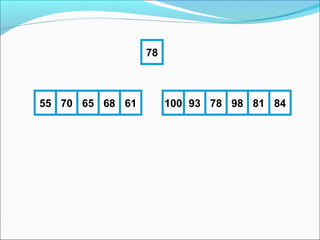
- 24. 78 70 65 84 98 78 100 93 55 61 81 68 78 70 65 84 98 78 100 93 55 61 81 68 78 70 65 84 98 78 100 93 55 61 81 68 78 70 65 68 98 78 100 93 55 61 81 84
- 25. 78 70 65 68 98 78 100 93 55 61 81 84 78 70 65 68 61 78 100 93 55 98 81 84 78 70 65 68 61 78 100 93 55 98 81 84 78 70 65 68 61 55 100 93 78 98 81 84 55 70 65 68 61 78 100 93 78 98 81 84
- 26. 78 55 70 65 68 61 100 93 78 98 81 84
- 27. Quicksort Implementation quicksort( void *a, int low, int high ) { int pivot; /* Termination condition! */ if ( high > low ) { pivot = partition( a, low, high ); quicksort( a, low, pivot-1 ); quicksort( a, pivot+1, high ); } } Divide Conquer
- 28. Quicksort - Partition int partition( int *a, int low, int high ) { int left, right; int pivot_item; pivot_item = a[low]; pivot = left = low; right = high; while ( left < right ) { /* Move left while item < pivot */ while( a[left] <= pivot_item ) left++; /* Move right while item > pivot */ while( a[right] >= pivot_item ) right--; if ( left < right ) SWAP(a,left,right); } /* right is final position for the pivot */ a[low] = a[right]; a[right] = pivot_item; return right; }
- 29. Quicksort - Partition This example uses int’s to keep things simple! int partition( int *a, int low, int high ) { int left, right; int pivot_item; pivot_item = a[low]; pivot = left = low; right = high; Any item will do as the pivot, while ( left < right ) { choose the leftmost one! /* Move left while item < pivot */ while( a[left] <= pivot_item ) left++; /* Move right while item > pivot */ while( a[right] >= pivot_item ) right--; if ( left < right ) SWAP(a,left,right); } 23 12 15 38 42 18 36 29 27 /* right is final position for the pivot */ a[low] = a[right]; a[right] = pivot_item; return right; low high }
- 30. Quicksort - Partition int partition( int *a, int low, int high ) { int left, right; int pivot_item; pivot_item = a[low]; pivot = left = low; Set left and right markers right = high; while ( left < right ) { /* Move left while item < pivot */ while( a[left] <= pivot_item ) left++; right left /* Move right while item > pivot */ while( a[right] >= pivot_item ) right--; if (23 12 right 38 SWAP(a,left,right);27 left < 15 ) 42 18 36 29 } /* right is final position for the pivot */ a[low]low a[right]; = high pivot: 23 a[right] = pivot_item; return right; }
- 31. Quicksort - Partition int partition( int *a, int low, int high ) { int left, right; int pivot_item; pivot_item = a[low]; pivot = left = low; right = high; Move the markers until they cross over while ( left < right ) { /* Move left while item < pivot */ while( a[left] <= pivot_item ) left++; /* Move right while item > pivot */ while( a[right] >= pivot_item ) right--; if ( left < right ) SWAP(a,left,right); left } /* right is final position for the pivot */ a[low] = a[right]; 15 38 42 18 36 29 23 12 a[right] = pivot_item; return right; low pivot: 23 } right 27 high
- 32. Quicksort - Partition int partition( int *a, int low, int high ) { int left, right; int pivot_item; pivot_item = a[low]; pivot = left = low; right = high; Move the left pointer while it points to items <= pivot while ( left < right ) { /* Move left while item < pivot */ while( a[left] <= pivot_item ) left++; /* Move right while item > pivot */ while( a[right] >= pivot_item ) right--; if ( left < right ) SWAP(a,left,right); left right } Move right /* right is final position for the pivot */ similarly a[low] = a[right]; 23 12 15 38 42 a[right] = pivot_item; 18 36 29 27 return right; } low high pivot: 23
- 33. Quicksort - Partition int partition( int *a, int low, int high ) { int left, right; int pivot_item; pivot_item = a[low]; pivot = left = low; right = high; Swap the two items on the wrong side of the pivot while ( left < right ) { /* Move left while item < pivot */ while( a[left] <= pivot_item ) left++; /* Move right while item > pivot */ while( a[right] >= pivot_item ) right--; if ( left < right ) SWAP(a,left,right); } left right /* right is final position for the pivot */ a[low] = a[right]; a[right] = pivot_item; 18 36 29 27 23 12 15 38 42 return right; pivot: 23 } low high
- 34. Quicksort - Partition int partition( int *a, int low, int high ) { int left, right; int pivot_item; pivot_item = a[low]; pivot = left = low; right = high; left and right have swapped over, so stop while ( left < right ) { /* Move left while item < pivot */ while( a[left] <= pivot_item ) left++; /* Move right while item > pivot */ while( a[right] >= pivot_item ) right--; if ( left < right ) SWAP(a,left,right); } right left /* right is final position for the pivot */ a[low] = a[right]; a[right] = pivot_item; 38 36 29 27 23 12 15 18 42 return right; } low high pivot: 23
- 35. Quicksort - Partition int partition( int *a, int low, int high ) { int left, right; int pivot_item; pivot_item = a[low]; pivot = left = low; right = high; right left while ( left < right ) { /* Move left while item < pivot */ 23 while( 18 42 38 36 29 27 12 15 a[left] <= pivot_item ) left++; /* Move right while item > pivot */ while( a[right] >= pivot_item ) right--; if ( left < right ) SWAP(a,left,right); low high pivot: 23 } /* right is final position for the pivot */ a[low] = a[right]; Finally, swap the pivot a[right] = pivot_item; and right return right; }
- 36. Quicksort - Partition int partition( int *a, int low, int high ) { int left, right; int pivot_item; pivot_item = a[low]; pivot = left = low; right = high; right while ( left < right ) { /* Move left while item < pivot */ 18 pivot: 23 while( 23 42 38 36 29 27 12 15 a[left] <= pivot_item ) left++; /* Move right while item > pivot */ while( a[right] >= pivot_item ) right--; if ( left < right ) SWAP(a,left,right); low high } /* right is final position for the pivot */ a[low] = a[right]; Return the position a[right] = pivot_item; of the pivot return right; }
- 37. Quicksort - Conquer pivot pivot: 23 18 12 15 Recursively sort left half 23 42 38 36 29 27 Recursively sort right half
- 39. Why study Heapsort? It is a well-known, traditional sorting algorithm you will be expected to know Heapsort is always O(n log n) Quicksort is usually O(n log n) but in the worst case slows to O(n2) Quicksort is generally faster, but Heapsort is better in time-critical applications Heapsort is a really cool algorithm!
- 40. What is a “heap”? Definitions of heap: 1. A large area of memory from which the programmer can allocate blocks as needed, and deallocate them (or allow them to be garbage collected) when no longer needed 2. A balanced, left-justified binary tree in which no node has a value greater than the value in its parent These two definitions have little in common Heapsort uses the second definition
- 41. Balanced binary trees Recall: The depth of a node is its distance from the root The depth of a tree is the depth of the deepest node A binary tree of depth n is balanced if all the nodes at depths 0 through n have two children n-2 n-1 n Balanced Balanced Not balanced
- 42. Left-justified binary trees A balanced binary tree is left-justified if: all the leaves are at the same depth, or all the leaves at depth n+1 are to the left of all the nodes at depth n Left-justified Not left-justified
- 43. Plan of attack First, we will learn how to turn a binary tree into a heap Next, we will learn how to turn a binary tree back into a heap after it has been changed in a certain way Finally (this is the cool part) we will see how to use these ideas to sort an array
- 44. The heap property A node has the heap property if the value in the node is as large as or larger than the values in its children 12 8 12 3 Blue node has heap property 8 12 12 Blue node has heap property 8 14 Blue node does not have heap property All leaf nodes automatically have the heap property A binary tree is a heap if all nodes in it have the heap property
- 45. shiftUp Given a node that does not have the heap property, you can give it the heap property by exchanging its value with the value of the larger child 12 8 14 14 Blue node does not have heap property 8 12 Blue node has heap property This is sometimes called shifting up Notice that the child may have lost the heap property
- 46. Constructing a heap I A tree consisting of a single node is automatically a heap We construct a heap by adding nodes one at a time: Add the node just to the right of the rightmost node in the deepest level If the deepest level is full, start a new level Examples: Add a new node here Add a new node here
- 47. Constructing a heap II Each time we add a node, we may destroy the heap property of its parent node To fix this, we sift up But each time we sift up, the value of the topmost node in the shift may increase, and this may destroy the heap property of its parent node We repeat the shifting up process, moving up in the tree, until either We reach nodes whose values don’t need to be swapped (because the parent is still larger than both children), or We reach the root
- 49. Other children are not affected 12 10 8 12 5 14 14 8 14 5 10 12 8 5 10 The node containing 8 is not affected because its parent gets larger, not smaller The node containing 5 is not affected because its parent gets larger, not smaller The node containing 8 is still not affected because, although its parent got smaller, its parent is still greater than it was originally
- 50. A sample heap Here’s a sample binary tree after it has been heapified 25 22 19 18 17 22 14 21 14 3 9 15 11 Notice that heapified does not mean sorted Heapifying does not change the shape of the binary tree; this binary tree is balanced and left-justified because it started out that way
- 51. Removing the root Notice that the largest number is now in the root Suppose we discard the root: 11 22 19 18 17 22 14 21 14 3 9 15 11 How can we fix the binary tree so it is once again balanced and left-justified? Solution: remove the rightmost leaf at the deepest level and use it for the new root
- 52. The reHeap method I Our tree is balanced and left-justified, but no longer a heap However, only the root lacks the heap property 11 22 19 18 17 22 14 21 14 3 15 9 We can shiftUp() the root After doing this, one and only one of its children may have lost the heap property
- 53. The reHeap method II Now the left child of the root (still the number 11) lacks the heap property 22 11 19 18 17 22 14 21 14 3 15 9 We can shiftUp() this node After doing this, one and only one of its children may have lost the heap property
- 54. The reHeap method III Now the right child of the left child of the root (still the number 11) lacks the heap property: 22 22 19 18 17 11 14 21 14 3 15 9 We can shiftUp() this node After doing this, one and only one of its children may have lost the heap property —but it doesn’t, because it’s a leaf
- 55. The reHeap method IV Our tree is once again a heap, because every node in it has the heap property 22 22 19 18 17 21 14 11 14 3 15 9 Once again, the largest (or a largest) value is in the root We can repeat this process until the tree becomes empty This produces a sequence of values in order largest to smallest
- 56. Sorting What do heaps have to do with sorting an array? Here’s the neat part: Because the binary tree is balanced and left justified, it can be represented as an array All our operations on binary trees can be represented as operations on arrays To sort: heapify the array; while the array isn’t empty { remove and replace the root; reheap the new root node; }
- 57. Mapping into an array 25 22 17 19 18 0 22 14 1 2 14 21 3 4 3 5 6 9 7 8 15 11 9 10 25 22 17 19 22 14 15 18 14 21 3 11 12 9 11 Notice: The left child of index i is at index 2*i+1 The right child of index i is at index 2*i+2 Example: the children of node 3 (19) are 7 (18) and 8 (14)
- 58. Removing and replacing the root The “root” is the first element in the array The “rightmost node at the deepest level” is the last element Swap them... 0 1 2 3 4 5 6 7 8 9 10 25 22 17 19 22 14 15 18 14 21 3 0 1 2 3 4 5 6 7 8 9 10 11 22 17 19 22 14 15 18 14 21 3 11 12 9 11 11 12 9 25 ...And pretend that the last element in the array no longer exists—that is, the “last index” is 11 (9)
- 59. Reheaproot node repeat and (index 0, containing Reheap the 0 1 2 3 4 5 6 7 8 9 10 11 22 17 19 22 14 15 18 14 21 3 0 1 2 3 4 5 6 7 8 9 10 22 22 17 19 21 14 15 18 14 11 3 0 1 2 3 4 5 6 7 8 9 10 11 11)... 12 9 25 11 12 9 25 11 12 9 22 17 19 22 14 15 18 14 21 3 22 25 ...And again, remove and replace the root node Remember, though, that the “last” array index is changed Repeat until the last becomes first, and the array is sorted!
- 60. Analysis I Here’s how the algorithm starts: heapify the array; Heapifying the array: we add each of n nodes Each node has to be shifted up, possibly as far as the root Since the binary tree is perfectly balanced, sifting up a single node takes O(log n) time Since we do this n times, heapifying takes n*O(log n) time, that is, O(n log n) time
- 61. Analysis II Here’s the rest of the algorithm: while the array isn’t empty { remove and replace the root; reheap the new root node; } We do the while loop n times (actually, n-1 times), because we remove one of the n nodes each time Removing and replacing the root takes O(1) time Therefore, the total time is n times however long it takes the reheap method
- 62. Analysis III To reheap the root node, we have to follow one path from the root to a leaf node (and we might stop before we reach a leaf) The binary tree is perfectly balanced Therefore, this path is O(log n) long And we only do O(1) operations at each node Therefore, reheaping takes O(log n) times Since we reheap inside a while loop that we do n times, the total time for the while loop is n*O(log n), or O(n log n)
- 63. Analysis IV Here’s the algorithm again: heapify the array; while the array isn’t empty { remove and replace the root; reheap the new root node; } We have seen that heapifying takes O(n log n) time The while loop takes O(n log n) time The total time is therefore O(n log n) + O(n log n) This is the same as O(n log n) time