SlideShare a Scribd company logo
SPATIAL POINT
PATTERNS
NYC Stop and Frisk.
Emerald Ash Borer
UFO Sightings.
Point Thinking
• Point pattern analysis is about finding and explaining
structure in maps of locations.
Point pattern terminology
• Point is the term used for an arbitrary location
• Event is the term used for an observation, events occur at
points.
!
• Window: Is our study region. The language is important here..
The word “window” implies that we are looking through glass at
a piece of a process.
!
• Mapped point pattern: A map of points, assumes all relevant
events w/in study area have been recorded
!
• Sampled point pattern: events are recorded from a sample of
different areas within a region
Point Thinking
Window
There are points out here too but we can’t see them
(because they are outside the window).
An alternate window
Both windows are views
of the same process
Point Thinking
• Point pattern analysis requires an odd mindset.
• The data you have is a single realization of…
• In point pattern analysis we view a map as a single realization of
some underlying probability surface.
• At each location there is some probability of an event occurring.
Point Thinking
• This probability is denoted λ (lambda).
• Often referred to as intensity.
• Point pattern analysis often involves assumptions about
intensity.
• or simple statistical models of intensity...
• We start simple….
• Analysis becomes more complex as assumptions/models
about intensity evolve.
Point Thinking
• The simplest assumption that we can make is the lambda
is constant.
• Lambda is said to be “homogenous” within the window.
• Implies that points are equally likely at all locations.
• The number of points in any location is a Poisson random variable.
• Random draw from a Poisson distribution with mean/variance = lambda
Poisson Point Process
1. We could divide our window into subregions (B)
2. The expected number of points in a subregion B is
simply λ* area(B).
3. As long as regions don't overlap the number of points in
B1 is completely independent from the number of points
in B2.
4. Finally, the location of points within B will be completely
random. The location of the first point has no effect
onthe location of the second point.
!
• If the above rules hold a point pattern is said to be a
uniform Poisson Point Process or to represent complete
spatial randomness (CSR).
Objective of point pattern analysis
• Did our data come from CSR process.
• Are event locations random? (humans are really bad at this…).
• Did some other process generate our data?
• Can we develop a model that explains the patterns in our data?
• Are locations random?
• That is there evidence that events interact with each other. For
example, do points attract or repulse each other?
• Do different types of points have a relationship to each
other?
• Are oak trees attracted or repulsed by pine trees?
• Where are significant clusters of events/points?
Find the clusters and gaps…
Types of relationships among points
• Three general patterns
• Random - any point is equally likely to occur at any location and the
position of any point is not affected by the position of any other point
• Uniform - every point is as far from all of its neighbors as possible
(repulsion).
• Clustered - many points are concentrated close together, and large
areas that contain very few, if any, points (attraction).
RANDOM UNIFORM
(REPULSION)
CLUSTERED
(ATTRACTION)
Types of distributions
Point patterns are scale specific.
• What looks like a clustered pattern at one scale can look
like a random (or dispersed pattern at another scale).
• Many point pattern analysis techniques are inherently
multiscale.
• Anytime the word “function” is in the title of a point pattern
techniques it implies the test is done as a function of distance.
• Thus, in point pattern analysis one find scale specific
patterns.
What kind of pattern?
Focal point
Two approaches…
• Exploring 1st order properties
• Measuring intensity (lambda)
• Use the density of points in an area
• Kernel estimation is used to describe variations in density.
• Even under CSR density will vary locally.
• We can derive images (raster maps) from maps of points.
• Are local variations in intensity more extreme or less extreme that we’d see under
CSR?
• Tested with a quadrant analysis.
• Exploring 2nd order properties
• Measuring spatial dependence
• Often called “distance methods.”
• Distances between points.
• Usually as a function of distance
• Nearest neighbor (G-Function)
• Number of points as a function of distance (K-function)
SPATIAL POINT PATTERNS
Kernel estimation
• Creating a smooth surface for each kernel
• Surface value highest in the center (point location) and
diminishes with distance…reaches 0 at radius distance
Kernel estimation
• s is a location in R (the study area)
• s1…sn are the locations of n events in R
!
• The intensity at a specific location is estimated by:
!
!
!
!
!
!
!
• Summed across all points si within the radius (τ)
!
"
#
$
%
& −
= ∑
= τ
τ
λτ
i
n
i
s
s
k
s
1
2
1
)
(
ˆ
kernel
(which is a function of the
distance and bandwidth)
bandwidth
(radius of the circle)
distance between
point s and si
Uniform
!
Triangular
!
Quartic
!
Gaussian
!
Different types of kernels
!
"
#
$
%
& −
= ∑
= τ
τ
λτ
i
n
i
s
s
k
s
1
2
1
)
(
ˆ
Each kernel type has a different
equation for the function k, for example:
!
Triangular:
!
!
!
Quartic:
!
!
!
Normal: 2
2
2
2
2
2
1
1
3
1
τ
π
τ
π
τ
i
h
i
i
e
k
h
k
d
k
−
=
$
$
%
&
'
'
(
)
−
=
−
=
Kernel estimation
• The kernel (k) is basically a mathematical function that
calculates how the surface value “falls off” as it reaches the
radius
• There are lots of different kernel functions
• Most researchers believe it doesn’t really matter which you use
• Most common in GIS is the quartic or gaussian kernel
!
!
!
!
!
!
!
• Summed for all values of di which are not larger than τ
• In practice the kind of kernel doesn’t matter – but the
bandwidth does.
2
2
2
2
1
3
)
(
ˆ
!
!
"
#
$
$
%
&
−
= ∑
< τ
πτ
λ
τ
τ
i
n
d
d
s
i
bandwidth
(radius of the circle)
distance between point s and si
At point s, the weight is
3/πτ2 and drops smoothly
to a value of 0 at τ
Kernel estimation
λ(s)
2
2
2
2
1
3
!
!
"
#
$
$
%
&
−
τ
πτ
i
d
2
2
2
2
1
3
!
!
"
#
$
$
%
&
−
∑
< τ
πτ
τ
i
n
d
d
i
Individual “bumps”
Adding up the “bumps”
Kernel Density (left) Source Data (right)
Calculating density in R.
• The best R-library for point pattern analysis is called
“spatstat” it is actively being developed.
• Most spatstat functions use a “ppp” object.
• ppp objects consist of coordinates, a window, and “marks” of
attribute data for each point.
• The function “density” when passed a ppp object
calculates a kernel density estimate (using a gaussian
kernel).
• We’ll go over the details in lab…
A few notes
• Points can be weighted.
• A point with a lot of deaths could be weighted so that it contributed
more the the resulting kernel density.
• However, this goes against the “event” logic of many point tests. An
event is discrete occurrence…
• Like GWR, we can use fixed and adaptive kernels
• Fixed = bandwidth is a specified distance
• Adaptive = fixed number of points used
• Results are sensitive to change in bandwidth
• When bandwidth is larger, the intensity will appear smooth and local
details obscured
• When bandwidth is small, the intensity appears as local spikes at
event locations
Using Images
• The result of calculating a kernel density surface is an
image.
• Images can be used in conjunction with points to do interesting
analysis.
• For example, we might have an image representing elevation.
• We might want to know how the intensity of trees varies with
elevation.
• Using the Iraq data, looking at the we might want to know
if places that have a high intensity of deaths have a high
intensity of “Friendly Action.”
Areas with more deaths saw more “friendly actions” (all friendly actions
in the data resulted in 1 or more deaths).
This map shows a weighted kernel density
for total deaths and friendly actions (marked w/ “x”)
G
r
a
p
h
s
u
m
m
a
r
i
z
e
s
m
a
p
HYPOTHESIS TESTING
Quadrat methods
• Divide the study area into subregions of equal size
• Often squares, but don’t have to be
• Count the frequency of events in each subregion
• Calculate the intensity of events in each subregion
Quadrat methods
Quadrat method
• Compare the variation in intensity over R
3 1
5 0
2 1
1 3
3 1
Quadrat
#
# of Points
Per Quadrat x^2
1 3 9
2 1 1
3 5 25
4 0 0
5 2 4
6 1 1
7 1 1
8 3 9
9 3 9
10 1 1
20 60
Variance 2.222
Mean 2.000
Var/Mean 1.111
2 2
2 2
2 2
2 2
2 2
Quadrat
#
# of Points
Per Quadrat x^2
1 2 4
2 2 4
3 2 4
4 2 4
5 2 4
6 2 4
7 2 4
8 2 4
9 2 4
10 2 4
20 40
Variance 0.000
Mean 2.000
Var/Mean 0.000
0 0
0 0
10 10
0 0
0 0
Quadrat
#
# of Points
Per Quadrat x^2
1 0 0
2 0 0
3 0 0
4 0 0
5 10 100
6 10 100
7 0 0
8 0 0
9 0 0
10 0 0
20 200
Variance 17.778
Mean 2.000
Var/Mean 8.889
To test for CSR we can examine the variance-mean ratio, values greater than
1 indicate clustering.
We can also do a chi-square test:
!
sum((observed-expected)^2/expected)
!
This is done in R with library spatstat via quadrat.test(aMap, nx=nXquads,
ny=nYquads).
Quadrats in R
!
Chi-squared test of CSR using
quadrat counts
!
data: id.sppp
X-squared = 94378.58, df = 5, p-
value < 2.2e-16
alternative hypothesis:
two.sided
!
Quadrats: 2 by 3 grid of tiles
Weaknesses of quadrat method
• Quadrat size
• If too small, they may contain only a couple of points
• If too large, they may contain too many points
• A rule of thumb is to use 2(area/n) quadrants
• Actually a measure of dispersion, and not really pattern,
because it is based primarily on the density of points, and
not their arrangement in relation to one another
!
• Results in a single measure for the entire distribution, so
variations within the region are not recognized
Nearest neighbor analysis
G-function
• Examine the cumulative frequency distribution of the
nearest neighbor distances
3
5
8
4
2
12 7
1
10
6
11
9
10 meters
Even
t x y
Nearest
neighbo
r
rmin
1 66.22 32.54 10 25.59
2 22.52 22.39 4 15.64
3 31.01 81.21 5 21.14
4 9.47 31.02 8 24.81
5 30.78 60.10 3 9.00
6 75.21 58.93 10 21.14
7 79.26 7.68 12 21.94
8 8.23 39.93 4 9.00
9 98.73 42.53 6 21.94
10 89.78 42.53 6 21.94
11 65.19 92.08 6 34.63
12 54.46 8.48 7 24.81
G-function
G(r) =
# point pairs where rmin ≤ r
# of points in study area
Even
t x y
Nearest
neighbo
r
rmin
1 66.22 32.54 10 25.59
2 22.52 22.39 4 15.64
3 31.01 81.21 5 21.14
4 9.47 31.02 8 24.81
5 30.78 60.10 3 9.00
6 75.21 58.93 10 21.14
7 79.26 7.68 12 21.94
8 8.23 39.93 4 9.00
9 98.73 42.53 6 21.94
10 89.78 42.53 6 21.94
11 65.19 92.08 6 34.63
12 54.46 8.48 7 24.81
G(r)
0
0.25
0.5
0.75
1
Distance (r)
0 9 15 22 25 26 35
G-function
The shape of G-function tells us the way the events are
spaced in a point pattern
• Clustered = G increases
rapidly at short distance
• Evenness = G increases
slowly up to distance where
most events spaced, then
increases rapidly
• How do we examine
significance (significant
departure from CSR)?
G(r)
0
0.25
0.5
0.75
1
Distance (r)
0 9 15 22 25 26 35
How do we tell if G is significant?
• The significance of any departures from CSR (either
clustering or regularity) can be evaluated using simulated
“confidence envelopes”
• Simulate many (1000??) spatial point processes and
estimate the G function for each of these
• Rank all the simulations
• Pull out the 5th and 95th G(r) values
• Plot these as the 95% confidence intervals
• This is done in R!
G(r) radius (r)
95th
5th
G estimate in R
!
> G <- envelope(a.ppp.object, Gest, nsim = 99)
> plot(G)
Grey area represents
The range of results
under CSR
The black line is our data.
More neighbors than expected…
What happens here?
Empty Space
F-function
• Select a sample of point locations anywhere in the study
region at random
• Determine minimum distance from each point to any event in the
study area
!
• Three steps:
1. Randomly select m points (p1, p2, …, pn)
2. Calculate dmin(pi, s) as the minimum distance from location pi to
any event in the point pattern s
3. Calculate F(d)
F-function (Empty Space Function)
F(d) =
# of point pairs where rmin ≤ r
# sample points
10 meters
= randomly chosen point
= event in study area
= dmin
F(r)
0
0.3
0.5
0.8
1
Distance (r)
0 5 10 15 20 25
F-function
• Clustered = F(r) rises
slowly at first, but more
rapidly at longer
distances
• Evenness = F(r) rises
rapidly at first, then
slowly at longer
distances
• Examine significance by
simulating “envelopes”
F(r)
0
0.3
0.5
0.8
1
Distance (r)
0 5 10 15 20 25
F estimate in R
➢F <- envelope(a.ppp.object, Fest, nsim = 99)
Empty spaces distances
larger than expected.
This is evidence of clustering
Comparison between G and F
K-Function
• Limitation of nearest neighbor distance and the empty
space test (G & F-functions) method is that they use only
nearest distance
• Considers only the shortest scales of variation
• K function (Ripley, 1976) uses more points
• Provides an estimate of spatial dependence over a wider range of
scales
• Based on all the distances between events in the study area.
K function
• Defined as:
!
!
!
!
• Lambda is the intensity of the pattern.
• Under CSR the number of points within a sub region is
constant.
• So we expect the number of points around an arbitrary point to be a
function of h.
• Where h is the radius of a circle centered on an arbitrary event.
How do we estimate the K-function
1.Construct a circle of radius h around each point event (i)
2.Count the number of other events (j) that fall inside this
circle
3.Repeat these two steps for all points (i) and sum results
!
!
!
!
!
!
!
4.Increment h by a small amount and repeat the computation
∑∑
≠
=
j
i ij
ij
h
w
d
I
n
R
h
K
)
(
)
(
ˆ
2
number of points
area of R
edge correction
the proportion of circumference of circle
(centered on point i, containing point j)
=1 if whole circle in the study area
Indicator variable = 1 if the
distance between points i and j
dij ≤ h, 0 otherwise
Estimate of intenstiy
SPATIAL POINT PATTERNS
Interpreting the K-function
• K(h) can be plotted against different values of h.
• As h increases, the area of the circles around each point increases.
• For constant intensity (CSR) the area of a subregion determines the
number of points.
• So K should increase with h…
!
• But what should K look like for violations of CSR?
• K above expectations
• More points than expected
• Evidence of clustering
• K below expectations
• Evidence of repulsion.
What does this show?
Clustering
Dispersion
Cross K-Functions
• An interesting extension of the K-Function is to consider
how many events of one type are located near a different
type of event.
• Are oak trees clustered near pine trees.
• This is different from asking if oak trees are clustered.
events
j
type
of
intensity
i)
point type
of
r
distance
j
type
of
points
E(#
1
)
(
j =
≤
=
λ
λj
ij d
K
Lansing Woods Data
• Location of trees of different species within a research plot
(a multi-type point pattern).
Cross K-Functions
Difference of K-Functions
• The difference between k-functions (K1 – K2) is a way to look for
differences between two point patterns for the same window.
• The cross k-function is about the relationships.
• How is this type of event distributed relative to that type of event?
• The difference between two highlights if one pattern is more or less
clustered than the other.
• Do these two types of events have the same pattern?
• If the event types have similar patterns we expect K1 – K2=0 for all
scales. Non-zero values signal difference.
• In spatstat there is existing function to get simulation envelope for
difference (I tried…).
Varying Intensity?
• The assumption that intensity does not vary within a study
is not realistic in some situations.
• Populations, soil types, slopes, these all vary spatially affecting the
distribution of observed patterns.
• We can visualize variations in intensity.
• We can also build models that account for these
variations.
Looking at relationships
• We might be interested in how the intensity varies with a
covariate.
• This implies that lambda varies spatially (with a covariate)
such that the intensity at location ui is not necessarily the
same as the intensity at location uj:
!
!
!
• For a covariate X at location u, we might be interested in:
Intensity and covariates
Intensity at location u
covariate
Some function that defines the association between
a covariate and intensity.
Intensity as a function of a covariate
• We might want to know if the intensity of points varies
systematically with a (continuous) covariate.
• This would imply inhomogeneity – that the intensity of the
point process was not constant.
• More importantly it would help us understand which factors
influence the intensity of events.
Inhomogeneous Point Processes
• Modeling variations in intensity.
• We do this with a raster image describing the factor(s) that cause
local variations in intensity:
• To build the raster image we build a model that predicts the intensity
of points.
• In spatstat this is called a point process model (ppm).
• A ppm is similar to a logistic model:
• ppm(bei, ~sl + el …) where bei is a map of points and sl
and el are covariates.
• The ~sl + el specify the log of the intensity function.
• For example this ppm model could include a dummy variable if intensity
was higher in one sum region of the map.
• For example a “soil suitability” dummy might be used to model the intensity of
trees.
• You can use AIC(MyPpm) to choose between ppm objects.
Point Process Model
• The resulting model can be used to simulate points and
displayed as an image.
• The dataset bei is included with R. It includes:
• The locations of a species of tree in a tropical research cite.
• An image of the elevation in the research site
• An image of the slope in the research site.
Slope and trees Elevation
Making a ppm
> data(bei)!
> bei.elev <- bei.extra$elev!
> bei.slope <- bei.extra$grad!
> ppm.bei <- ppm(bei, ~sl + el,
! covariates=list(sl=bei.slope, el=bei.elev))!
> coefs(ppm.bei)!
(Intercept) sl el !
-8.55862210 5.84104065 0.02140987 !
!
> plot(predict.ppm(ppm.bei, type="lambda"),
main="Predicted Intensity (lambda)")
SPATIAL POINT PATTERNS
Using a ppm.
• To simulate points using a ppm a
process called “independent thinning is
used”
• We have Poisson process X with
intensity, λ and that each point of X is
either deleted or retained.
• Then points are deleted from X with
probability p(u) where p(u) is the output
from a ppm.
• For simulation a useful technique is
independent thinning. If the retention
probability at location u is p(u), then the
resulting process of retained points is
Poisson, with intensity function λ’(u) =
λ*p(u), for all u.
• To see what this looks like you can
type:
aMap <- simulate(myPPM)
plot(aMap)
Modeling inhomogeneous processes
• Make our own point generating process.
• It is a poission process but the intensity for each location varies
• Create simulated maps based on the ppm.
• Calculate a k-function for the simulated ppm.
• Do the above two steps a lot of times, this will give you an envelope.
• Calculate a k-function for your real data. See if it fits within the envelope
created via the ppm simulation.
• If the “real” k-function fits within the envelope of the simulated
ppm k-functions then you have “explained” the observed
distribution of points.
• In this case a “significant” results means we have not
successfully modeled the underlying intensity surface for our
data.
• More in the lab exercise.
Beyond Inhomogeneous Poisson Processes
• Even this sophisticated approach assumes that the
location of points are independent.
• The next step in complexity is to create processes with explicit
interactions between points.
• For example, a Neyman-Scott Process is one in which a Poisson
process generates initial points and then a secondary Poisson
process generates points near those initial points.
• Imagine a tree dropping seeds…

More Related Content

What's hot (20)

PPT
Image quality assessment and statistical evaluation
DocumentStory
 
PPTX
Principal component analysis
Farah M. Altufaili
 
PPTX
Spatial Autocorrelation
Ehsan Hamzei
 
PPT
Digital image classification22oct
Aleemuddin Abbasi
 
PPTX
Principal Component Analysis (PCA) and LDA PPT Slides
AbhishekKumar4995
 
PPTX
Steps for Principal Component Analysis (pca) using ERDAS software
Swetha A
 
PDF
Principles of GIS unit 2
SanjanaKhemka1
 
PDF
Visualizing Data Using t-SNE
David Khosid
 
PPTX
Introduction to principal component analysis (pca)
Mohammed Musah
 
PDF
Image classification
Anchor Charan
 
PPTX
Pca ppt
Dheeraj Dwivedi
 
PPTX
Lect5 principal component analysis
hktripathy
 
PPTX
Gis functions
Shah Naseer
 
PPTX
Spectral Clustering
ssusered887b
 
PDF
Spatial Data Science with R
amsantac
 
PPT
3.7 outlier analysis
Krish_ver2
 
PPTX
GIS Geographical Information System
Muhammad Hamza Khan KaimKhani
 
PDF
Exploratory data analysis
gokulprasath06
 
PPTX
Introduction to GIS
Obaidur Rahaman Ovi
 
PPTX
Geographic Information System unit 1
sridevi5983
 
Image quality assessment and statistical evaluation
DocumentStory
 
Principal component analysis
Farah M. Altufaili
 
Spatial Autocorrelation
Ehsan Hamzei
 
Digital image classification22oct
Aleemuddin Abbasi
 
Principal Component Analysis (PCA) and LDA PPT Slides
AbhishekKumar4995
 
Steps for Principal Component Analysis (pca) using ERDAS software
Swetha A
 
Principles of GIS unit 2
SanjanaKhemka1
 
Visualizing Data Using t-SNE
David Khosid
 
Introduction to principal component analysis (pca)
Mohammed Musah
 
Image classification
Anchor Charan
 
Lect5 principal component analysis
hktripathy
 
Gis functions
Shah Naseer
 
Spectral Clustering
ssusered887b
 
Spatial Data Science with R
amsantac
 
3.7 outlier analysis
Krish_ver2
 
GIS Geographical Information System
Muhammad Hamza Khan KaimKhani
 
Exploratory data analysis
gokulprasath06
 
Introduction to GIS
Obaidur Rahaman Ovi
 
Geographic Information System unit 1
sridevi5983
 

Similar to SPATIAL POINT PATTERNS (20)

PDF
GIS in Public Health Research: Understanding Spatial Analysis and Interpretin...
hpaocec
 
PDF
Finding Meaning in Points, Areas and Surfaces: Spatial Analysis in R
Revolution Analytics
 
PDF
Autocorrelation_kriging_techniques for Hydrology
smartwateriitrk
 
PPT
GEOSTATISTICAL_ANALYST
Putu Santikayasa
 
PPTX
Building maps with analysis
LindaBeale
 
PDF
Introduction to spatstat
Richard Wamalwa
 
PPTX
Basic geostatistics
Serdar Kaya
 
PDF
Spatial interpolation comparison
Tomislav Hengl
 
PPT
geostatistics_for introduction and analysis
GadisaGeremewNegasa
 
PPTX
Classification Systems
John Reiser
 
PPT
Lecture8 clustering
sidsingh680
 
PDF
Pami meanshift
irisshicat
 
PDF
Student_Garden_geostatistics_course
Pedro Correia
 
PDF
Student_Garden_geostatistics_course
Pedro Correia
 
PDF
CLIM Fall 2017 Course: Statistics for Climate Research, Geostats for Large Da...
The Statistical and Applied Mathematical Sciences Institute
 
PPTX
Geostatistics for spatia data analysis and interpretaion.pptx
MariamKariam1
 
PDF
SCA_Module Supply Chain Data Analytics Supply Chain Data Analytics Supply Cha...
MujtabaAliKhan12
 
PPT
dm_spdm_short.ppt
SahilShahPhD2020
 
PPT
dm_spdm_short (3).ppt
yakot2alordea2
 
PDF
Introduction geostatistic for_mineral_resources
Adi Handarbeni
 
GIS in Public Health Research: Understanding Spatial Analysis and Interpretin...
hpaocec
 
Finding Meaning in Points, Areas and Surfaces: Spatial Analysis in R
Revolution Analytics
 
Autocorrelation_kriging_techniques for Hydrology
smartwateriitrk
 
GEOSTATISTICAL_ANALYST
Putu Santikayasa
 
Building maps with analysis
LindaBeale
 
Introduction to spatstat
Richard Wamalwa
 
Basic geostatistics
Serdar Kaya
 
Spatial interpolation comparison
Tomislav Hengl
 
geostatistics_for introduction and analysis
GadisaGeremewNegasa
 
Classification Systems
John Reiser
 
Lecture8 clustering
sidsingh680
 
Pami meanshift
irisshicat
 
Student_Garden_geostatistics_course
Pedro Correia
 
Student_Garden_geostatistics_course
Pedro Correia
 
CLIM Fall 2017 Course: Statistics for Climate Research, Geostats for Large Da...
The Statistical and Applied Mathematical Sciences Institute
 
Geostatistics for spatia data analysis and interpretaion.pptx
MariamKariam1
 
SCA_Module Supply Chain Data Analytics Supply Chain Data Analytics Supply Cha...
MujtabaAliKhan12
 
dm_spdm_short.ppt
SahilShahPhD2020
 
dm_spdm_short (3).ppt
yakot2alordea2
 
Introduction geostatistic for_mineral_resources
Adi Handarbeni
 
Ad

Recently uploaded (20)

PPTX
apidays Helsinki & North 2025 - API access control strategies beyond JWT bear...
apidays
 
PPTX
apidays Helsinki & North 2025 - Running a Successful API Program: Best Practi...
apidays
 
PDF
Avatar for apidays apidays PRO June 07, 2025 0 5 apidays Helsinki & North 2...
apidays
 
PPT
Data base management system Transactions.ppt
gandhamcharan2006
 
PDF
The European Business Wallet: Why It Matters and How It Powers the EUDI Ecosy...
Lal Chandran
 
PPTX
apidays Helsinki & North 2025 - From Chaos to Clarity: Designing (AI-Ready) A...
apidays
 
PDF
R Cookbook - Processing and Manipulating Geological spatial data with R.pdf
OtnielSimopiaref2
 
PPTX
AI Presentation Tool Pitch Deck Presentation.pptx
ShyamPanthavoor1
 
PDF
List of all the AI prompt cheat codes.pdf
Avijit Kumar Roy
 
PDF
Early_Diabetes_Detection_using_Machine_L.pdf
maria879693
 
PDF
Choosing the Right Database for Indexing.pdf
Tamanna
 
PDF
WEF_Future_of_Global_Fintech_Second_Edition_2025.pdf
AproximacionAlFuturo
 
PDF
apidays Helsinki & North 2025 - Monetizing AI APIs: The New API Economy, Alla...
apidays
 
PPTX
apidays Singapore 2025 - From Data to Insights: Building AI-Powered Data APIs...
apidays
 
PPTX
ER_Model_with_Diagrams_Presentation.pptx
dharaadhvaryu1992
 
PDF
Building Production-Ready AI Agents with LangGraph.pdf
Tamanna
 
PPT
Growth of Public Expendituuure_55423.ppt
NavyaDeora
 
PPTX
apidays Helsinki & North 2025 - Vero APIs - Experiences of API development in...
apidays
 
PPTX
apidays Helsinki & North 2025 - Agentic AI: A Friend or Foe?, Merja Kajava (A...
apidays
 
PDF
Web Scraping with Google Gemini 2.0 .pdf
Tamanna
 
apidays Helsinki & North 2025 - API access control strategies beyond JWT bear...
apidays
 
apidays Helsinki & North 2025 - Running a Successful API Program: Best Practi...
apidays
 
Avatar for apidays apidays PRO June 07, 2025 0 5 apidays Helsinki & North 2...
apidays
 
Data base management system Transactions.ppt
gandhamcharan2006
 
The European Business Wallet: Why It Matters and How It Powers the EUDI Ecosy...
Lal Chandran
 
apidays Helsinki & North 2025 - From Chaos to Clarity: Designing (AI-Ready) A...
apidays
 
R Cookbook - Processing and Manipulating Geological spatial data with R.pdf
OtnielSimopiaref2
 
AI Presentation Tool Pitch Deck Presentation.pptx
ShyamPanthavoor1
 
List of all the AI prompt cheat codes.pdf
Avijit Kumar Roy
 
Early_Diabetes_Detection_using_Machine_L.pdf
maria879693
 
Choosing the Right Database for Indexing.pdf
Tamanna
 
WEF_Future_of_Global_Fintech_Second_Edition_2025.pdf
AproximacionAlFuturo
 
apidays Helsinki & North 2025 - Monetizing AI APIs: The New API Economy, Alla...
apidays
 
apidays Singapore 2025 - From Data to Insights: Building AI-Powered Data APIs...
apidays
 
ER_Model_with_Diagrams_Presentation.pptx
dharaadhvaryu1992
 
Building Production-Ready AI Agents with LangGraph.pdf
Tamanna
 
Growth of Public Expendituuure_55423.ppt
NavyaDeora
 
apidays Helsinki & North 2025 - Vero APIs - Experiences of API development in...
apidays
 
apidays Helsinki & North 2025 - Agentic AI: A Friend or Foe?, Merja Kajava (A...
apidays
 
Web Scraping with Google Gemini 2.0 .pdf
Tamanna
 
Ad

SPATIAL POINT PATTERNS

  • 2. NYC Stop and Frisk.
  • 5. Point Thinking • Point pattern analysis is about finding and explaining structure in maps of locations.
  • 6. Point pattern terminology • Point is the term used for an arbitrary location • Event is the term used for an observation, events occur at points. ! • Window: Is our study region. The language is important here.. The word “window” implies that we are looking through glass at a piece of a process. ! • Mapped point pattern: A map of points, assumes all relevant events w/in study area have been recorded ! • Sampled point pattern: events are recorded from a sample of different areas within a region
  • 7. Point Thinking Window There are points out here too but we can’t see them (because they are outside the window). An alternate window Both windows are views of the same process
  • 8. Point Thinking • Point pattern analysis requires an odd mindset. • The data you have is a single realization of… • In point pattern analysis we view a map as a single realization of some underlying probability surface. • At each location there is some probability of an event occurring.
  • 9. Point Thinking • This probability is denoted λ (lambda). • Often referred to as intensity. • Point pattern analysis often involves assumptions about intensity. • or simple statistical models of intensity... • We start simple…. • Analysis becomes more complex as assumptions/models about intensity evolve.
  • 10. Point Thinking • The simplest assumption that we can make is the lambda is constant. • Lambda is said to be “homogenous” within the window. • Implies that points are equally likely at all locations. • The number of points in any location is a Poisson random variable. • Random draw from a Poisson distribution with mean/variance = lambda
  • 11. Poisson Point Process 1. We could divide our window into subregions (B) 2. The expected number of points in a subregion B is simply λ* area(B). 3. As long as regions don't overlap the number of points in B1 is completely independent from the number of points in B2. 4. Finally, the location of points within B will be completely random. The location of the first point has no effect onthe location of the second point. ! • If the above rules hold a point pattern is said to be a uniform Poisson Point Process or to represent complete spatial randomness (CSR).
  • 12. Objective of point pattern analysis • Did our data come from CSR process. • Are event locations random? (humans are really bad at this…). • Did some other process generate our data? • Can we develop a model that explains the patterns in our data? • Are locations random? • That is there evidence that events interact with each other. For example, do points attract or repulse each other? • Do different types of points have a relationship to each other? • Are oak trees attracted or repulsed by pine trees? • Where are significant clusters of events/points?
  • 13. Find the clusters and gaps…
  • 14. Types of relationships among points • Three general patterns • Random - any point is equally likely to occur at any location and the position of any point is not affected by the position of any other point • Uniform - every point is as far from all of its neighbors as possible (repulsion). • Clustered - many points are concentrated close together, and large areas that contain very few, if any, points (attraction).
  • 16. Point patterns are scale specific. • What looks like a clustered pattern at one scale can look like a random (or dispersed pattern at another scale). • Many point pattern analysis techniques are inherently multiscale. • Anytime the word “function” is in the title of a point pattern techniques it implies the test is done as a function of distance. • Thus, in point pattern analysis one find scale specific patterns.
  • 17. What kind of pattern?
  • 18. What kind of pattern?
  • 20. Two approaches… • Exploring 1st order properties • Measuring intensity (lambda) • Use the density of points in an area • Kernel estimation is used to describe variations in density. • Even under CSR density will vary locally. • We can derive images (raster maps) from maps of points. • Are local variations in intensity more extreme or less extreme that we’d see under CSR? • Tested with a quadrant analysis. • Exploring 2nd order properties • Measuring spatial dependence • Often called “distance methods.” • Distances between points. • Usually as a function of distance • Nearest neighbor (G-Function) • Number of points as a function of distance (K-function)
  • 22. Kernel estimation • Creating a smooth surface for each kernel • Surface value highest in the center (point location) and diminishes with distance…reaches 0 at radius distance
  • 23. Kernel estimation • s is a location in R (the study area) • s1…sn are the locations of n events in R ! • The intensity at a specific location is estimated by: ! ! ! ! ! ! ! • Summed across all points si within the radius (τ) ! " # $ % & − = ∑ = τ τ λτ i n i s s k s 1 2 1 ) ( ˆ kernel (which is a function of the distance and bandwidth) bandwidth (radius of the circle) distance between point s and si
  • 24. Uniform ! Triangular ! Quartic ! Gaussian ! Different types of kernels ! " # $ % & − = ∑ = τ τ λτ i n i s s k s 1 2 1 ) ( ˆ Each kernel type has a different equation for the function k, for example: ! Triangular: ! ! ! Quartic: ! ! ! Normal: 2 2 2 2 2 2 1 1 3 1 τ π τ π τ i h i i e k h k d k − = $ $ % & ' ' ( ) − = − =
  • 25. Kernel estimation • The kernel (k) is basically a mathematical function that calculates how the surface value “falls off” as it reaches the radius • There are lots of different kernel functions • Most researchers believe it doesn’t really matter which you use • Most common in GIS is the quartic or gaussian kernel ! ! ! ! ! ! ! • Summed for all values of di which are not larger than τ • In practice the kind of kernel doesn’t matter – but the bandwidth does. 2 2 2 2 1 3 ) ( ˆ ! ! " # $ $ % & − = ∑ < τ πτ λ τ τ i n d d s i bandwidth (radius of the circle) distance between point s and si At point s, the weight is 3/πτ2 and drops smoothly to a value of 0 at τ
  • 27. Kernel Density (left) Source Data (right)
  • 28. Calculating density in R. • The best R-library for point pattern analysis is called “spatstat” it is actively being developed. • Most spatstat functions use a “ppp” object. • ppp objects consist of coordinates, a window, and “marks” of attribute data for each point. • The function “density” when passed a ppp object calculates a kernel density estimate (using a gaussian kernel). • We’ll go over the details in lab…
  • 29. A few notes • Points can be weighted. • A point with a lot of deaths could be weighted so that it contributed more the the resulting kernel density. • However, this goes against the “event” logic of many point tests. An event is discrete occurrence… • Like GWR, we can use fixed and adaptive kernels • Fixed = bandwidth is a specified distance • Adaptive = fixed number of points used • Results are sensitive to change in bandwidth • When bandwidth is larger, the intensity will appear smooth and local details obscured • When bandwidth is small, the intensity appears as local spikes at event locations
  • 30. Using Images • The result of calculating a kernel density surface is an image. • Images can be used in conjunction with points to do interesting analysis. • For example, we might have an image representing elevation. • We might want to know how the intensity of trees varies with elevation. • Using the Iraq data, looking at the we might want to know if places that have a high intensity of deaths have a high intensity of “Friendly Action.”
  • 31. Areas with more deaths saw more “friendly actions” (all friendly actions in the data resulted in 1 or more deaths). This map shows a weighted kernel density for total deaths and friendly actions (marked w/ “x”) G r a p h s u m m a r i z e s m a p
  • 33. Quadrat methods • Divide the study area into subregions of equal size • Often squares, but don’t have to be • Count the frequency of events in each subregion • Calculate the intensity of events in each subregion
  • 35. Quadrat method • Compare the variation in intensity over R
  • 36. 3 1 5 0 2 1 1 3 3 1 Quadrat # # of Points Per Quadrat x^2 1 3 9 2 1 1 3 5 25 4 0 0 5 2 4 6 1 1 7 1 1 8 3 9 9 3 9 10 1 1 20 60 Variance 2.222 Mean 2.000 Var/Mean 1.111 2 2 2 2 2 2 2 2 2 2 Quadrat # # of Points Per Quadrat x^2 1 2 4 2 2 4 3 2 4 4 2 4 5 2 4 6 2 4 7 2 4 8 2 4 9 2 4 10 2 4 20 40 Variance 0.000 Mean 2.000 Var/Mean 0.000 0 0 0 0 10 10 0 0 0 0 Quadrat # # of Points Per Quadrat x^2 1 0 0 2 0 0 3 0 0 4 0 0 5 10 100 6 10 100 7 0 0 8 0 0 9 0 0 10 0 0 20 200 Variance 17.778 Mean 2.000 Var/Mean 8.889 To test for CSR we can examine the variance-mean ratio, values greater than 1 indicate clustering. We can also do a chi-square test: ! sum((observed-expected)^2/expected) ! This is done in R with library spatstat via quadrat.test(aMap, nx=nXquads, ny=nYquads).
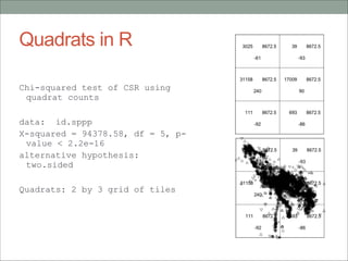
  • 37. Quadrats in R ! Chi-squared test of CSR using quadrat counts ! data: id.sppp X-squared = 94378.58, df = 5, p- value < 2.2e-16 alternative hypothesis: two.sided ! Quadrats: 2 by 3 grid of tiles
  • 38. Weaknesses of quadrat method • Quadrat size • If too small, they may contain only a couple of points • If too large, they may contain too many points • A rule of thumb is to use 2(area/n) quadrants • Actually a measure of dispersion, and not really pattern, because it is based primarily on the density of points, and not their arrangement in relation to one another ! • Results in a single measure for the entire distribution, so variations within the region are not recognized
  • 39. Nearest neighbor analysis G-function • Examine the cumulative frequency distribution of the nearest neighbor distances 3 5 8 4 2 12 7 1 10 6 11 9 10 meters Even t x y Nearest neighbo r rmin 1 66.22 32.54 10 25.59 2 22.52 22.39 4 15.64 3 31.01 81.21 5 21.14 4 9.47 31.02 8 24.81 5 30.78 60.10 3 9.00 6 75.21 58.93 10 21.14 7 79.26 7.68 12 21.94 8 8.23 39.93 4 9.00 9 98.73 42.53 6 21.94 10 89.78 42.53 6 21.94 11 65.19 92.08 6 34.63 12 54.46 8.48 7 24.81
  • 40. G-function G(r) = # point pairs where rmin ≤ r # of points in study area Even t x y Nearest neighbo r rmin 1 66.22 32.54 10 25.59 2 22.52 22.39 4 15.64 3 31.01 81.21 5 21.14 4 9.47 31.02 8 24.81 5 30.78 60.10 3 9.00 6 75.21 58.93 10 21.14 7 79.26 7.68 12 21.94 8 8.23 39.93 4 9.00 9 98.73 42.53 6 21.94 10 89.78 42.53 6 21.94 11 65.19 92.08 6 34.63 12 54.46 8.48 7 24.81 G(r) 0 0.25 0.5 0.75 1 Distance (r) 0 9 15 22 25 26 35
  • 41. G-function The shape of G-function tells us the way the events are spaced in a point pattern • Clustered = G increases rapidly at short distance • Evenness = G increases slowly up to distance where most events spaced, then increases rapidly • How do we examine significance (significant departure from CSR)? G(r) 0 0.25 0.5 0.75 1 Distance (r) 0 9 15 22 25 26 35
  • 42. How do we tell if G is significant? • The significance of any departures from CSR (either clustering or regularity) can be evaluated using simulated “confidence envelopes” • Simulate many (1000??) spatial point processes and estimate the G function for each of these • Rank all the simulations • Pull out the 5th and 95th G(r) values • Plot these as the 95% confidence intervals • This is done in R! G(r) radius (r) 95th 5th
  • 43. G estimate in R ! > G <- envelope(a.ppp.object, Gest, nsim = 99) > plot(G) Grey area represents The range of results under CSR The black line is our data. More neighbors than expected… What happens here?
  • 44. Empty Space F-function • Select a sample of point locations anywhere in the study region at random • Determine minimum distance from each point to any event in the study area ! • Three steps: 1. Randomly select m points (p1, p2, …, pn) 2. Calculate dmin(pi, s) as the minimum distance from location pi to any event in the point pattern s 3. Calculate F(d)
  • 45. F-function (Empty Space Function) F(d) = # of point pairs where rmin ≤ r # sample points 10 meters = randomly chosen point = event in study area = dmin F(r) 0 0.3 0.5 0.8 1 Distance (r) 0 5 10 15 20 25
  • 46. F-function • Clustered = F(r) rises slowly at first, but more rapidly at longer distances • Evenness = F(r) rises rapidly at first, then slowly at longer distances • Examine significance by simulating “envelopes” F(r) 0 0.3 0.5 0.8 1 Distance (r) 0 5 10 15 20 25
  • 47. F estimate in R ➢F <- envelope(a.ppp.object, Fest, nsim = 99) Empty spaces distances larger than expected. This is evidence of clustering
  • 49. K-Function • Limitation of nearest neighbor distance and the empty space test (G & F-functions) method is that they use only nearest distance • Considers only the shortest scales of variation • K function (Ripley, 1976) uses more points • Provides an estimate of spatial dependence over a wider range of scales • Based on all the distances between events in the study area.
  • 50. K function • Defined as: ! ! ! ! • Lambda is the intensity of the pattern. • Under CSR the number of points within a sub region is constant. • So we expect the number of points around an arbitrary point to be a function of h. • Where h is the radius of a circle centered on an arbitrary event.
  • 51. How do we estimate the K-function 1.Construct a circle of radius h around each point event (i) 2.Count the number of other events (j) that fall inside this circle 3.Repeat these two steps for all points (i) and sum results ! ! ! ! ! ! ! 4.Increment h by a small amount and repeat the computation ∑∑ ≠ = j i ij ij h w d I n R h K ) ( ) ( ˆ 2 number of points area of R edge correction the proportion of circumference of circle (centered on point i, containing point j) =1 if whole circle in the study area Indicator variable = 1 if the distance between points i and j dij ≤ h, 0 otherwise Estimate of intenstiy
  • 53. Interpreting the K-function • K(h) can be plotted against different values of h. • As h increases, the area of the circles around each point increases. • For constant intensity (CSR) the area of a subregion determines the number of points. • So K should increase with h… ! • But what should K look like for violations of CSR? • K above expectations • More points than expected • Evidence of clustering • K below expectations • Evidence of repulsion.
  • 54. What does this show? Clustering Dispersion
  • 55. Cross K-Functions • An interesting extension of the K-Function is to consider how many events of one type are located near a different type of event. • Are oak trees clustered near pine trees. • This is different from asking if oak trees are clustered. events j type of intensity i) point type of r distance j type of points E(# 1 ) ( j = ≤ = λ λj ij d K
  • 56. Lansing Woods Data • Location of trees of different species within a research plot (a multi-type point pattern).
  • 58. Difference of K-Functions • The difference between k-functions (K1 – K2) is a way to look for differences between two point patterns for the same window. • The cross k-function is about the relationships. • How is this type of event distributed relative to that type of event? • The difference between two highlights if one pattern is more or less clustered than the other. • Do these two types of events have the same pattern? • If the event types have similar patterns we expect K1 – K2=0 for all scales. Non-zero values signal difference. • In spatstat there is existing function to get simulation envelope for difference (I tried…).
  • 59. Varying Intensity? • The assumption that intensity does not vary within a study is not realistic in some situations. • Populations, soil types, slopes, these all vary spatially affecting the distribution of observed patterns. • We can visualize variations in intensity. • We can also build models that account for these variations.
  • 60. Looking at relationships • We might be interested in how the intensity varies with a covariate. • This implies that lambda varies spatially (with a covariate) such that the intensity at location ui is not necessarily the same as the intensity at location uj: ! ! ! • For a covariate X at location u, we might be interested in:
  • 61. Intensity and covariates Intensity at location u covariate Some function that defines the association between a covariate and intensity.
  • 62. Intensity as a function of a covariate • We might want to know if the intensity of points varies systematically with a (continuous) covariate. • This would imply inhomogeneity – that the intensity of the point process was not constant. • More importantly it would help us understand which factors influence the intensity of events.
  • 63. Inhomogeneous Point Processes • Modeling variations in intensity. • We do this with a raster image describing the factor(s) that cause local variations in intensity: • To build the raster image we build a model that predicts the intensity of points. • In spatstat this is called a point process model (ppm). • A ppm is similar to a logistic model: • ppm(bei, ~sl + el …) where bei is a map of points and sl and el are covariates. • The ~sl + el specify the log of the intensity function. • For example this ppm model could include a dummy variable if intensity was higher in one sum region of the map. • For example a “soil suitability” dummy might be used to model the intensity of trees. • You can use AIC(MyPpm) to choose between ppm objects.
  • 64. Point Process Model • The resulting model can be used to simulate points and displayed as an image. • The dataset bei is included with R. It includes: • The locations of a species of tree in a tropical research cite. • An image of the elevation in the research site • An image of the slope in the research site. Slope and trees Elevation
  • 65. Making a ppm > data(bei)! > bei.elev <- bei.extra$elev! > bei.slope <- bei.extra$grad! > ppm.bei <- ppm(bei, ~sl + el, ! covariates=list(sl=bei.slope, el=bei.elev))! > coefs(ppm.bei)! (Intercept) sl el ! -8.55862210 5.84104065 0.02140987 ! ! > plot(predict.ppm(ppm.bei, type="lambda"), main="Predicted Intensity (lambda)")
  • 67. Using a ppm. • To simulate points using a ppm a process called “independent thinning is used” • We have Poisson process X with intensity, λ and that each point of X is either deleted or retained. • Then points are deleted from X with probability p(u) where p(u) is the output from a ppm. • For simulation a useful technique is independent thinning. If the retention probability at location u is p(u), then the resulting process of retained points is Poisson, with intensity function λ’(u) = λ*p(u), for all u. • To see what this looks like you can type: aMap <- simulate(myPPM) plot(aMap)
  • 68. Modeling inhomogeneous processes • Make our own point generating process. • It is a poission process but the intensity for each location varies • Create simulated maps based on the ppm. • Calculate a k-function for the simulated ppm. • Do the above two steps a lot of times, this will give you an envelope. • Calculate a k-function for your real data. See if it fits within the envelope created via the ppm simulation. • If the “real” k-function fits within the envelope of the simulated ppm k-functions then you have “explained” the observed distribution of points. • In this case a “significant” results means we have not successfully modeled the underlying intensity surface for our data. • More in the lab exercise.
  • 69. Beyond Inhomogeneous Poisson Processes • Even this sophisticated approach assumes that the location of points are independent. • The next step in complexity is to create processes with explicit interactions between points. • For example, a Neyman-Scott Process is one in which a Poisson process generates initial points and then a secondary Poisson process generates points near those initial points. • Imagine a tree dropping seeds…