Spectral Clustering Report

Spectral Clustering
Miaolan Xie
February 9, 2015
1 INTRODUCTION
Spectral clustering is the problem of finding clusters using spectral algorithms. Clustering is a
very useful technique widely used in scientific research areas involving empirical data. As it is a
natural question to ask, given a big set of data, if we can put the data into groups such that data in
the same group has similar behavior. Spectral clustering often outperforms traditional clustering
algorithms, as it does not make strong assumptions on the form of the clusters. In addition, it is
easy to implement, and can be efficiently solved by standard linear algebra software.
In this chapter, we will focus on studying spectral clustering algorithms, and this chapter is
mainly based on the survey paper by Ulrike von Luxburg (2007). We will first get familiar with
the background materials related to spectral clustering, and then see two basic spectral algorithms.
Afterwards, we will try to get some intuition on these spectral algorithms: why the algorithms are
designed as they are. We try to rigorously justify the algorithms from graph cut point of view,
perturbation theory point of view. Another theoretical justification will be given for a slightly
modified spectral algorithm. Lastly, some practical details and issues will be discussed.
1.1 Background materials
Intuitively clustering is the problem of dividing data into groups, so that data points in the same
group are more similar to each other than to those in other groups. We care about clustering
problem since it gives a first impression of the data being analyzed, and is widely used in any
scientific field dealing with empirical data. However, clustering is in general a hard problem. It is
already NP-hard to cluster a set of vectors in a Euclidean space.
Spectral clustering is the problem of finding clusters by spectral algorithms. The basic idea is
the following: First, define a graph G that captures the properties of the original data set. Then,
use certain eigenvectors of a certain Laplacian of the graph G to form clusters. There are several
advantages of spectral clustering: it is simple to implement and runs efficiently. Furthermore, it
often outperforms traditional clustering algorithms.
Before we can run any spectral clustering algorithm on the data set, we first need to measure
the ”similarities” sij between each pair of data points xi, xj. We may use distance function to
define the pairwise similarity: assign the similarity sij to be big if the distance between xi and xj
is small, and assign a small similarity if their distance is big. Details will be discussed in Section
Six. There are other ways to define the similarity function as well.
With the data and their pairwise similarity given, we can now define a similarity graph G =
(V, E) of the data set using these information. We want this weighted graph to capture properties
1

of the original data. It can be defined as follows: assign a vertex vi to each data point xi, create
an edge between vi and vj if their similarity sij is positive or bigger than a certain threshold, and
take the similarity sij to be the weight of each edge vivj created.
With the similarity graph, the original clustering problem is now turned into a graph partition
problem. Since finding a grouping of the original data set such that different groups are dissimilar
to each other in terms of similarity graph is finding a partition of the similarity graph such that
the edges going between different groups have low weights.
1.2 Notations
Here are some notations that will be used later for similarity graph G = (V, E), V = {v1, ..., vn}:
• non-negative weight of vivj is defined as wij.
• W := (wij)i,j=1,.,n is the weighted adjacency matrix of the graph G.
• di := n
j=1 wij denotes the degree of vi.
• D denotes the diagonal degree matrix of G, with Dii = di for i ∈ {1, ..., n}.
• ¯A denotes the complement of vertex set A.
• W(A, B) := i∈A,j∈B wij is the sum of the weights of all edges going between set A and B.
• vol(A) := i∈A di is a measure of the size of set A.
• |A|:= the cardinality of A is another measure of the size of set A.
• 1Ai denotes the indicator vector of set Ai.
1.3 Different ways to construct the similarity graph
There are other ways to construct similarity graph of a data set in addition to the one described
before:
• Fully connected graph: this similarity graph is the one described above, we create an edge
between two points if their similarity sij is positive. Set wij = sij if vivj ∈ E.
• -neighborhood graph: connect two points if their pairwise distance is smaller than . This
graph is usually treated as an unweighted graph, since if vivj ∈ E, the distance between xi
and xj is roughly of the same scale as .
• k-nearest neighbor graph: for each vertex vi, connect it to all of its k-nearest neighbors. Since
this relation is not symmetric, we obtain a directed graph. The k-nearest neighbor graph is
obtained by simply ignoring the directions on the edges, and set wij = sij if vivj ∈ E.
• Mutual k-nearest neighbor graph: is similar to k-nearest neighbor graph. The only difference
is that after the directed graph is created, only keep edges that are bidirected, and ignore the
directions. An undirected graph is obtained in this way. Set wij = sij if vivj ∈ E.
2

1.4 Review of graph Laplacians
Before getting into the spectral clustering algorithms, let’s briefly review graph Laplacians and
their basic properties:
I. Unnormalized Laplacian
The unnormalized Laplacian L is defined as L = D − W. Some basic properties are as follows:
1. fT Lf = 1
2
n
i,j=1 wij(fi − fj)2 holds for any f ∈ Rn.
2. L has n non-negative real eigenvalues: 0 = λ1 ≤ λ2 ≤ ... ≤ λn.
3. The smallest eigenvalue of L is 0, and the corresponding eigenvector is 1.
4. The number of connected components A1, ..., Ak in graph G equals to the number of eigen-
values of L equal to 0, and the eigenspace of eigenvalue 0 is spanned by vectors 1A1 , ..., 1Ak
.
II. Normalized Laplacian
For our purpose, we define normalized Laplacian slightly differently here: Lrw = D−1L =
I − D−1W. It is denoted as Lrw, since it is related to the random walk matrix.
It is straightforward to verify the following properties also hold for Lrw:
1. Lrwu = λu if and only if λ and u solve the generalized eigenproblem Lu = λDu.
2. Lrw has n non-negative real eigenvalues: 0 = λ1 ≤ λ2 ≤ ... ≤ λn.
3. The smallest eigenvalue of Lrw is 0, and the corresponding eigenvector is 1.
4. The number of connected components A1, ..., Ak in graph G equals to the number of eigen-
values of Lrw equal to 0, and the eigenspace of eigenvalue 0 is spanned by vectors 1A1 , ..., 1Ak
.
2 SPECTRAL CLUSTERING ALGORITHMS
Now, we are ready to see two basic spectral clustering algorithms. The first algorithm uses unnor-
malized Laplacian, and the second one uses normalized Laplacian. The two algorithms are very
similar to each other, and the only difference is they use different graph Laplacians. However, us-
ing different graph Laplacians may lend to different outcomes of clustering. We will discuss which
algorithm is more preferable at the end of Section Six.
2.1 Two basic spectral clustering algorithms
Before running the spectral clustering algorithms, first measure the pairwise similarities sij for each
pair of data xi and xj. Form similarity matrix S = (sij)i,j=1...n.
A basic unnormalized spectral clustering algorithm is as follows:
3

Unnormalized Spectral Clustering Algorithm
Input: Similarity matrix S ∈ Rn×n
, number k of clusters to construct.
1. Construct a similarity graph by one of the ways described before.
Let W be its weighted adjacency matrix.
2. Compute the unnormalized Laplacian L.
3. Compute the first k eigenvectors u1, ..., uk of L.
4. Let U ∈ Rn×k
be the matrix containing the vectors u1, ..., uk as columns.
5. For i = 1, ..., n, let yi ∈ Rk
be the vector corresponding to the i-th row of U.
6. Cluster the points (yi)i=1,...,n in Rk
with k-means algorithm to obtain clusters C1, ..., Ck.
Output: Clusters A1, ..., Ak with Ai = {j|yj ∈ Ci}.
There are different versions of normalized spectral clustering algorithms. A basic one by Shi
and Malik (2000) is as follows:
Normalized Spectral Clustering Algorithm according to Shi and Malik (2000)
Input: Similarity matrix S ∈ Rn×n
, number k of clusters to construct.
1. Construct a similarity graph by one of the ways described before.
Let W be its weighted adjacency matrix.
2. Compute the unnormalized Laplacian L.
3. Compute the first k eigenvectors u1, ..., uk of the generalized eigenproblem Lu = λDu.
4. Let U ∈ Rn×k
be the matrix containing the vectors u1, ..., uk as columns.
5. For i = 1, ..., n, let yi ∈ Rk
be the vector corresponding to the i-th row of U.
6. Cluster the points (yi)i=1,...,n in Rk
with k-means algorithm to obtain clusters C1, ..., Ck.
We see the only difference between these two algorithms is step 3. For normalized clustering
algorithm, the first k eigenvectors of the generalized eigenproblem Lu = λDu are exactly the first k
eigenvectors of the normalized Laplacian Lrw if D is invertible (by the first property of normalized
Laplacian). Thus, essentially the only difference between these two algorithms is they use different
Laplacians to obtain the first k eigenvectors. The reason the normalized algorithm does not use
Lrw directly is that Lrw is not defined when D is not invertible.
Note that the number of clusters k to be constructed is an input of the algorithms. Unfortu-
nately, in general it is not an easy task to figure out the appropriate k. A useful heuristic will be
discussed in Section Six.
In both algorithms, each row of the matrix U is a vector in the Euclidean space Rk. We think
of each row vector of U as a vector representation of one data point. In other words, we obtain an
embedding of the original data set in Rk by making use of the first k eigenvectors of the Laplacian.
We hope this is a meaningful embedding, and when the last step of the algorithms (i.e., the k-means
clustering step) is performed on this vector embedding, a clustering can be easily identified and it
induces a good clustering of the original data set. We will see this is indeed the case.
4

Figure 1: A toy example
2.2 The k-means algorithm
For completeness, we briefly introduce the k-means algorithm as in the last step of the spectral
clustering algorithms.
Given a set of n vectors, k-means clustering problem aims to partition the vectors into k sets,
S = {S1, ...Sk} such that the partition minimizes the within-cluster sum of squares:
min:
k
i=1 xj∈Si
xj − ui
2
, where ui is the mean of vectors in Si.
k-means clustering is a NP-hard problem.
The k-means algorithm stated below is a widely used heuristic algorithm for k-means clustering.
It is an iterative algorithm, and finds a clustering by the Euclidean distances between vectors. The
algorithm is as follows:
k-means algorithm:
Input: n vectors, number k of clusters to be constructed.
1. Randomly pick k vectors as the initial group centers.
2. Assign each vector to its closest center, and obtain a grouping.
3. Recalculate the centers by taking means of the groups.
4. Repeat step 2 & 3 until the centers no longer move. (i.e., the group assignment no longer
changes)
In general, this algorithm runs efficiently, but there are cases the algorithm converges very
slowly.
2.3 Illustrate by a toy example
Let’s consider a toy example to get some intuition on the spectral clustering algorithms.
Suppose a similarity graph of the original data points is constructed as in Figure 1, each edge in
the graph has weight 1, and the input parameter k is chosen to be 3. Clearly, we hope the spectral
5

clustering algorithms return three clusters: {1, 2, 3}, {4, 5, 6}, and {7, 8, 9}. Let’s step through the
algorithms:
Since the similarity graph has three components, by property 4 of both Laplacians, the first 3
eigenvalues are all equal to 0, and the first 3 eigenvectors are all linear combinations of 1{1,2,3}, 1{4,5,6}
and 1{7,8,9}. As a result, all three eigenvectors are constant on {1, 2, 3}, {4, 5, 6}, and {7, 8, 9} en-
tries. Thus, the matrix U must have the form of:














a1 a2 a3
a1 a2 a3
a1 a2 a3
b1 b2 b3
b1 b2 b3
b1 b2 b3
c1 c2 c3
c1 c2 c3
c1 c2 c3














.
As discussed before, each row of this matrix is a vector representation of a data point, so we see
data points 1, 2, 3 are represented by the same vector (a1, a2, a3) in R3, 4, 5, 6 are all represented by
(b1, b2, b3), and 7, 8, 9 are all represented by (c1, c2, c3). Moreover, since the three eigenvectors span
a 3-dimensional space, (a1, a2, a3), (b1, b2, b3) and (c1, c2, c3) must be three distinct points in R3.
Now, if we apply the k-means clustering algorithm on this vector embedding of the data points, we
will trivially get each of the three vectors as one cluster in R3. This clustering in R3 induces the
clustering of {1, 2, 3}, {4, 5, 6}, and {7, 8, 9} of the original data set, which is exactly the correct
clustering.
By this toy example, we see the spectral algorithms do seem to capture certain fundamental
properties of clustering.
2.4 Intuitive justification for spectral algorithms
The toy example above provides some intuitive idea why the spectral algorithms make sense. In
this section, some additional intuitive justification is given.
Compare the following two facts:
• A graph G is disconnected if and only if there exist at least 2 eigenvalues of the
Laplacians equal to 0. (Fact 1)
This fact follows directly from the last property of both Laplacians.
• a graph G has a sparse cut if and only if there exist at least 2 eigenvalues of the
Laplacians close to 0. (Fact 2)
This fact follows from Cheeger’s inequality. Cheeger’s inequality shows that the graph con-
ductance can be approximated by the second eigenvalue of the Laplacian. In other words, a
graph has a small conductance if and only if the second eigenvalue of the graph Laplacian is
small. Thus, Fact 2 follows.
It is obvious that Fact 2 is an approximate version of Fact 1.
Naturally, we may ask if there is an analogous characterization for an arbitrary k. It turns out
this is indeed the case. In the paper by Lee, Oveis Gharan and Trevisan (2012), it is shown that a
graph G can be partitioned into k sparse cuts if and only if there exist k eigenvalues close to 0.
6

This shows the small eigenvalues and their eigenvectors have some strong connection with the
sparse partitioning of a graph. Hence, it does make sense to use the first k eigenvectors to find
clustering of the data set.
3 GRAPH CUT POINT OF VIEW
The previous section gives some intuitive justification for the spectral algorithms. Now, let’s see
some rigorous justification. The first rigorous justification is from graph cut point of view.
As discussed before, with the similarity graph constructed, we turned the clustering problem
into a graph partition problem. Instead of finding a clustering so that data points in the same cluster
are similar to each other and points in different clusters are dissimilar to each other, we want to
find a partition of the graph so that edges within a group have big weights, and edges between
different groups have small weights. We will see spectral clustering algorithms are approximation
algorithms to graph partition problems.
Let’s first define the graph partition problem mathematically. Since the goal is to find a partition
A1, ..., Ak of the graph so that there are very few edges going between different groups, we can choose
the objective function to be total weights of all cut edges: cut(A1, ..., Ak):= 1
2
k
i=1 W(Ai, ¯Ai). The
scalar of 1
2 is due to the fact every cut edge is counted twice when summing over all group cuts.
Thus, the graph partition problem is defined as: arg min
A1,...,Ak
: Cut(A1, ..., Ak).
Notice when k equals to 2, this problem is exactly the minimum cut problem. There exist
efficient algorithms for this problem. However, in practice running the minimum cut algorithm in
many cases only ends up separating a single vertex from the rest of the graph. This is not what we
want since we want the clusters to be reasonably large sets of points.
To fix this, we require the partition to be not only sparse but balanced as well. This can be
achieved by explicitly incorporating these requirements into the objective function. Instead of using
total weights of cut edges as the objective function, consider RatioCut and Ncut functions as follows:
RatioCut(A1, ..., Ak):= k
i=1
W(Ai, ¯Ai)
|Ai| = k
i=1
cut(Ai, ¯Ai)
|Ai| .
Ncut(A1, ..., Ak):= k
i=1
W(Ai, ¯Ai)
vol(Ai) = k
i=1
cut(Ai, ¯Ai)
vol(Ai) .
The difference between the Cut function and RatioCut, Ncut functions is that in RatioCut and
Ncut, each term in the sum is divided by the size of the group. The size of the group is measured
by the group cardinality in RatioCut, while in Ncut, the size of the group is measured by the
group volume. In this way, the requirement of having a balanced partition is incorporated into the
problem as well.
Thus, we consider these two graph partition problems instead:
RatioCut graph partition problem: arg min
A1,...,Ak
: RatioCut(A1, ..., Ak).
Ncut graph partition problem: arg min
A1,...,Ak
: Ncut(A1, ..., Ak).
However, with these two objective functions the graph partition problems become NP-hard.
The best we can hope for is to solve these problems approximately. Indeed, we will prove later
that the unnormalized spectral clustering algorithm solves the relaxed RatioCut problem and the
7

normalized spectral clustering algorithm solves the relaxed Ncut problem. This provides a formal
justification for the spectral algorithms.
3.1 Approximating RatioCut
In this section, we will prove the unnormalized spectral clustering algorithm solves relaxed RatioCut
problem.
The RatioCut problem is to find a partition that optimizes: min
A1,...,Ak
RatioCut(A1, ..., Ak). It
can be rewritten in the following way:
Represent each partition A1, ..., Ak by a matrix H = (h1|...|hk) ∈ Rn×k, where:
(hj)i =
1/ |Aj| if vi ∈ Aj
0 otherwise
j ∈ {1, ..., k}; i ∈ {1, ..., n} ( )
By definition, it is straightforward to check that {h1, ..., hk} is an orthonormal set. This implies
HT H = I.
It is also easy to check the following equality:
hT
i Lhi =
cut(Ai, ¯Ai)
|Ai|
(1)
Proof of equality (1):
hT
i Lhi =
1
2
n
k,l=1
wkl(hik − hil)2
=
1
2
k∈Ai,l∈ ¯Ai
wkl(
1
|Ai|
− 0)2
+
1
2
k∈ ¯Ai,l∈Ai
wkl(0 −
1
|Ai|
)2
=
1
2
cut(Ai, ¯Ai)(
1
|Ai|
) +
1
2
cut(Ai, ¯Ai)(
1
|Ai|
)
=
cut(Ai, ¯Ai)
|Ai|
.
Equality (2) below is easily verifiable as well:
hT
i Lhi = (HT
LH)ii (2)
With these two equalities and by definition of the trace function, we get:
RatioCut(A1, ..., Ak) = k
i=1 hT
i Lhi = k
i=1(HT LH)ii = Tr(HT LH).
Thus the problem: min
A1,...,Ak
RatioCut(A1, ..., Ak) can be rewritten as:
min
H∈Rn×k
Tr(HT LH) s.t. HT H = I, H as defined in ( ) for each partition.
Clearly, this is still an optimization problem over a discrete set, so it is still NP-hard. The
simplest way to relax the problem is to discard the discreteness:
min
H∈Rn×k
Tr(HT LH) s.t. HT H = I. This is the relaxed RatioCut problem.
8

Now, let’s show the unnormalized spectral clustering algorithm solves this relaxed RatioCut.
By a version of the Rayleigh-Ritz theorem, we know a matrix U having the first k eigenvectors
of L as its columns is an optimal solution of the relaxation. Hence, the matrix U constructed in
the unnormalized spectral algorithm is an optimal solution of the relaxation.
To obtain a partition from the optimal U, we consider the following two cases:
If U is one of the matrices defined as in ( ) for a graph partition, then by similar arguments as
in the toy example in Section Two, the unnormalized algorithm will return precisely the partition
corresponding to U as the grouping when we apply the k-means step on the rows of matrix U. In
this case, clearly this partition is an optimal solution for the original RatioCut problem. Thus, the
unnormalized algorithm solves the RatioCut problem exactly.
However, in general the optimal U is not one of the matrices defined for the graph partitions.
In this case, we can still run the k-means step on the rows of U to obtain a partition. Hopefully,
the partition returned is close to the optimal partition of the original RatioCut problem. Thus, the
unnormalized algorithm solves the RatioCut problem approximately in this case.
Now we can conclude that the unnormalized spectral clustering algorithm solves the relaxed
RatioCut problem. Note when k equals to 2, the spectral clustering algorithm coincides with the
algorithm derived from the proof of the Cheeger’s inequality.
3.2 Approximating Ncut
Similarly we can prove that the normalized spectral clustering algorithm solves the relaxed Ncut
problem. The proof is exactly analogous to the proof of the unnormalized spectral clustering
algorithm.
In this case, we represent each partition A1, ..., Ak by a matrix H = (h1|...|hk) ∈ Rn×k, where
(hj)i =
1/ vol(Aj) if vi ∈ Aj
0 otherwise
j ∈ {1, ..., k}; i ∈ {1, ..., n}.
The rest of the proof follows in a similar fashion as in the previous section.
3.3 Comments on the relaxation approach
First note that there is no guarantee on the quality of the solution of the relaxed problem (i.e.,
the solution returned by the spectral algorithm) compared to the optimal solution of the original
problem. In general, the objective difference between the two solutions can be arbitrarily large.
Such example can be found in section 5.4 of von Luxburg (2007). On the other hand, we note that
it is NP-hard to approximate any balanced graph partition problem with a constant approximation
ratio.
There exist other relaxations for the RatioCut and Ncut problem. The relaxations shown in the
previous sections are by no means unique. There are, for example, SDP relaxations as well. The
advantage of the spectral relaxation is that it results in a standard linear algebra problem which is
simple to solve.
9

4 PERTURBATION THEORY POINT OF VIEW
In this section, we rigorously justify the spectral algorithms from perturbation theory point of
view. Perturbation theory is the study of how eigenvalues and eigenvectors change when a small
perturbation is introduced to the matrix.
Intuitively, the justification by this approach is the following:
In the ideal situation, the similarity graph constructed represents the clustering structure of the
data exactly. In this case, each connected component of the similarity graph precisely corresponds
to one cluster of the original data set. With the ideal similarity graph, suppose the graph has k
components, the spectral algorithms will return k clusters corresponding to the k connected com-
ponents (by similar arguments as in the toy example). Clearly, in this case the spectral algorithms
produce the correct clustering.
However, in real life we may not always be able to construct the ideal similarity graph. The
graph constructed in real life is in general some perturbed version of the ideal graph. As a result, the
Laplacians of this similarity graph are perturbed versions of the ideal Laplacians. By perturbation
theory, if the perturbation is not too big and the eigengap between λk and λk+1 of the ideal
Laplacian is relatively large, then the first k eigenvectors of the perturbed Laplacian is ”close to”
the first k eigenvectors of the ideal one. Thus, in real life the matrix U constructed in the algorithms
is ”close to” the U in the ideal case. Thus, although in this case we may not have all points in a
cluster being represented by the same vector, their vector representations are still relatively close
to each other. Hence, after running the k-means step, the correct clustering can still be identified.
4.1 The rigorous perturbation argument
The above intuitive arguments can be made rigorous by Davis-Kahan theorem in perturbation
theory. Let’s first define some mathematical notions that are used in the theorem.
To measure the difference between two k-dimensional eigenspaces of symmetric matrices, prin-
cipal angles θi, i ∈ {1, ..., k} are generally used. They are defined as follows:
Suppose S1 and S2 are two k-dimensional subspaces of Rn and V1 and V2 are two matrices such
that their columns form orthonormal bases for S1 and S2, then the principal angles θi, i ∈ {1, ..., k}
are defined by taking the singular values of V T
1 V2 as the cosines cos(θi), i ∈ {1, ..., k}. Note that
when k equals to 1, this definition reduces to the normal angle definition between two lines in a
vector space.
The matrix sinΘ(S1, S2) is defined as:



sin(θ1) . . . 0
...
...
...
0 . . . sin(θk)


. We will use the Frobenius
norm of this matrix to measure the distance between subspaces S1 and S2. It is a reasonable
measure, since the bigger the angles between the subspaces, the bigger the norm will be.
Now, we can state the Davis-Kahan theorem:
Theorem 4.1. Davis-Kahan: Let A, H ∈ Rn×n be symmetric matrices, . be the Frobenius norm
of matrices, and Ã be A + H. Let I1 be an interval in R, σI1 (A) be the set of eigenvalues of A
in I1, and S1 be the corresponding eigenspace for these eigenvalues of A. Let ˜S1 be the analogous
eigenspace for Ã, δ := min{|λ − s|; λ eigenvalue of A, λ ∈ I1, s ∈ I1} be the smallest distance
between I1 and the eigenvalues of A outside of I1, and let the distance between subspaces S1 and ˜S1
be d(S1, ˜S1) := sinΘ(S1, ˜S1) , then the distance d(S1, ˜S1) ≤ H
δ .
10

For our purpose, we may think of the matrix A as the ideal Laplacian L (the normalized case
is similar), H as a perturbation matrix, and Ã as the Laplacian ˜L obtained in real life with some
”noise” H. Due to noise, the graph may not be completely disconnected on different clusters, but
different clusters are connected by edges with low weights. In our case, we choose the interval I1 so
that the first k eigenvalues of L and ˜L are all in the interval. Thus, S1 is the eigenspace spanned
by the first k eigenvectors of L, and ˜S1 is the eigenspace spanned by the first k eigenvectors of ˜L.
δ is the distance between I1 and λk+1 of L. If I1 can be chosen as [0, λk], then δ equals to the
eigengap between λk and λk+1. If the perturbation H is small, and the eigengap is large, then by
Davis-Kahan theorem we have the eigenspace S1 and ˜S1 close to each other (since their distance is
bounded by H
δ ).
By the same argument as before, we see the clustering the algorithm will return is close to
the true clustering. By the derivation, we see the smaller the perturbation H and the bigger the
spectral gap, the better the spectral algorithm works. Hence, we obtained another justification for
the spectral clustering algorithms.
5 JUSTIFICATION BY A SLIGHTLY MODIFIED SPECTRAL
ALGORITHM
Another justification for spectral clustering is provided in this section, and it is based on the paper
by Dey, Rossi and Sidiropoulos (2014). We will consider a slightly modified spectral clustering
algorithm as follows:
Input: Similarity matrix S ∈ Rn×n, number k of clusters to construct.
1. Construct a similarity graph by one of the ways described before. Let W be its weighted
adjacency matrix.
2. Compute the normalized Laplacian Lrw.
3. Compute the first k eigenvectors u1, ..., uk of Lrw.
4. Let U ∈ Rn×k be the matrix containing the vectors u1, ..., uk as columns.
5. For i = 1, ..., n, let yi ∈ Rk be the vector corresponding to the i-th row of U. Let f(vi) = yi.
6. Let R be a non-negative number (see Table 1 below), V0 = V (G).
7. For i = 1, ..., k − 1, let vi be the vertex in Vi−1 such that the ball centered at f(vi) with
radius 2R has the most number of vectors of f(Vi−1), set Ci = ball(f(vi), 2R)∩f(Vi−1), and update
Vi = Vi−1 Ci by removing previously chosen clusters.
8. Set Ck = Vk.
The only difference between this spectral clustering algorithm and the ones we have seen in
Section Two is that instead of using the k-means algorithm to obtain a clustering in the vector
space, an approximation algorithm (by Charikar et al. 2001) for the robust k-center problem is
used here.
11

Table 1:
R = (1 − 2k
√
δ)/(8k
√
n)
δ = 1/n + (c 3k3log3n)/τ
= maximum degree of graph G
c > 0 is a universal constant
τ > c 2k5log3n, and λ3
k+1(Lrw) > τλk(Lrw)
5.1 Justification for this spectral clustering algorithm
The paper by Dey, Rossi and Sidiropoulos shows that for a bounded-degree graph with |λk+1 − λk|
(of the normalized Laplacian) large enough, this algorithm returns a partition arbitrarily close to
a ”strong” one. A partition of a graph is strong if each group has small external conductance and
large internal conductance, which precisely characterizes a good clustering of the data set. Thus,
this is another theoretical justification for spectral clustering.
The high level intuition of the paper is as follows: (for detailed theorem statements and proofs
please see Dey, Rossi and Sidiropoulos, 2014)
By Oveis Gharan and Trevisan (2014), if the normalized Laplacian of a graph G has its eigengap
|λk+1 − λk| large enough, then there exists a graph partition into k groups, such that each group
has small external conductance and large internal conductance, i.e., the partition is strong.
To prove the claim that the above algorithm returns a partition arbitrarily close to a strong
one, two steps are needed. Step one involves showing that (given |λk+1 − λk| is large) for each of
the first k eigenvectors ui of the Laplacian, there exists a ˜ui close to ui, such that ˜ui is constant on
each group of the desired partition. Using step one, step two involves showing that (with the same
assumptions) in the embedding induced by the first k eigenvectors, most groups from the desired
strong partition are concentrated around center points in Rk, and different centers are sufficiently
far apart from each other. Thus, when we run the approximation algorithm for the robust k-center
problem, a partition arbitrarily close to a strong one is returned, so the claim follows.
5.2 Comments on this approach
Note this approach has similar flavor as the perturbation theory approach.
An experimental evaluation is carried out in the last section of the paper. Different graphs and
different k’s are chosen to exam whether the above algorithm returns reasonable clusters. It turns
out the algorithm returns meaningful clusters in all these cases, and the experiments suggest that
weaker assumptions may be used in the theorems. For a complete description of the experimental
result please see the paper.
Furthermore, we see from this algorithm, there is nothing principle in using the k-means algo-
rithm as the last step for spectral algorithms. If the graph is well constructed, after the data points
are embedded in the vector space, they will have well-expressed clusters so that every reasonable
clustering algorithm for vectors can identify them correctly. In addition to the approximation al-
gorithm for the robust k-center problem, there are many other techniques can be used in the last
step.
12

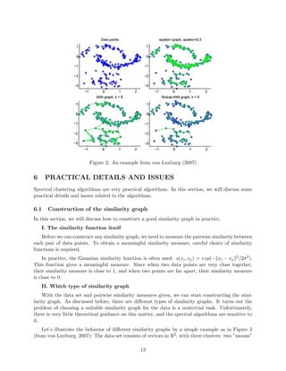
Figure 2: An example from von Luxburg (2007)
6 PRACTICAL DETAILS AND ISSUES
Spectral clustering algorithms are very practical algorithms. In this section, we will discuss some
practical details and issues related to the algorithms.
6.1 Construction of the similarity graph
In this section, we will discuss how to construct a good similarity graph in practice.
I. The similarity function itself
Before we can construct any similarity graph, we need to measure the pairwise similarity between
each pair of data points. To obtain a meaningful similarity measure, careful choice of similarity
functions is required.
In practice, the Gaussian similarity function is often used: s(xi, xj) = exp(− xi − xj
2/2σ2).
This function gives a meaningful measure. Since when two data points are very close together,
their similarity measure is close to 1, and when two points are far apart, their similarity measure
is close to 0.
II. Which type of similarity graph
With the data set and pairwise similarity measures given, we can start constructing the simi-
larity graph. As discussed before, there are diﬀerent types of similarity graphs. It turns out the
problem of choosing a suitable similarity graph for the data is a nontrivial task. Unfortunately,
there is very little theoretical guidance on this matter, and the spectral algorithms are sensitive to
it.
Let’s illustrate the behavior of diﬀerent similarity graphs by a simple example as in Figure 2
(from von Luxburg, 2007): The data set consists of vectors in R2, with three clusters: two ”moons”
13

at top and a Gaussian at bottom shown in the upper left panel of Figure 2. The Gaussian is chosen
to have a smaller density than that of the two moons.
The upper right panel shows the -neighborhood graph constructed using equals to 0.3. We see
the points in the two moons are relatively well connected to the clusters they belong to. However,
points in the Gaussian are barely connected to each other. As a result, when a spectral algorithm is
run on this graph, the two moon clusters may be identified correctly, but the Gaussian will not be
identified correctly. This is a general problem of -neighborhood graph: it is hard to fix a parameter
which works for a data set ”on different scales”.
The bottom left panel shows the k-nearest neighbor graph, with k equals to 5. Clearly, this
graph is well connected. The points are all connected to their respective clusters, and there are few
edges going between different clusters. Generally, k-nearest neighbor graph can deal with data on
different scales. Note the resulting Laplacians of this graph are sparse matrices, since by definition
there are at most k edges adjacent to any vertex.
The bottom right panel shows the mutual k-nearest neighbor graph. We see the connectivity
of this graph is somehow in between that of the previous two graphs. The Laplacian of the mutual
k-nearest neighbor graph is sparse as well.
We try to avoid the use of fully connected graph, since the Laplacian of a fully connected graph
is not sparse, so it will be computationally expensive.
In general, a well-connected similarity graph is preferred if it is not clear whether the dis-
connected components correspond to the correct clusters. Thus, the k-nearest neighbor graph is
suggested as the first choice in general.
6.2 Computing the eigenvectors
It is seen from the last section that the Laplacian matrices of many similarity graphs are sparse.
As seen in previous chapters, there exist efficient methods to compute the first k eigenvectors of
a sparse matrix. For example, some popular ones include the power method and Krylov subspace
methods. The speed of convergence of these methods depends on the eigengap |λk+1 − λk| of the
Laplacian. The larger the eigengap, the faster the convergence.
6.3 The number of clusters
As discussed before, the number k of clusters to construct is an input of the algorithms. In other
words, we need to determine the number of clusters to construct before we run the algorithms.
This turns out to be not an easy task.
This problem is not specifically for spectral clustering algorithms. It is a general problem for
all clustering algorithms. There are many heuristics, and the eigengap heuristic is particularly
designed for spectral clustering. It is the following: choose the number k such that λ1, ..., λk are
all very small, but λk+1 is relatively large.
Let’s illustrate why this heuristic makes sense by an example (from von Luxburg, 2007) as
in the figure below. On top left, the histogram shows a data set that clearly has four clusters.
We construct the 10-nearest neighbor graph of the data set and compute the eigenvalues of the
normalized Laplacian of the graph. The eigenvalues are plotted below the histogram. We see
the first four eigenvalues are all very close to 0, and there is a relatively big jump from λ4 to
λ5. By eigengap heuristic, this gap indicates the data set may have four clusters. The data set
14

represented by the histogram on top right does not seem to have any clear clusters, and the plot
of the eigenvalues also does not have any big eigengap, which coincides with our observation. This
example shows that there is indeed some fundamental connection between the number of clusters
in data set and big eigengap in the spectrum of Laplacian. Hence, this heuristic is justified.
6.4 Which Laplacian to use?
First note that if the similarity graph is nearly regular, using different Laplacians will not affect
the outcome much. Since for a regular graph, the unnormalized Laplacian and the normalized
Laplacian are only different by a multiple of identity matrix.
However, in general we encourage the use of normalized Laplacian. The reason is the following:
the goal of clustering is to find clusters with small between-cluster similarity and big within-cluster
similarity. In terms of similarity graph, we want a partition with small cut(Ai, ¯Ai) and big vol(Ai)
for each i ∈ {1, ..., k}. Observe that the Ncut graph partition problem encodes these requirements
exactly since the Ncut objective is Ncut(A1, ..., Ak) = k
i=1
cut(Ai, ¯Ai)
vol(Ai) . Moreover, the normalized
spectral clustering algorithm solves the relaxed Ncut problem (as proved previously), so it makes
sense to use normalized Laplacian to find clustering. Note that the unnormalized algorithm solves
the relaxed RatioCut, but the RatioCut objective requires |Ai| instead of vol(Ai) to be small, which
is not quite what we want. Hence, the use of normalized Laplacian is encouraged in general.
7 CONCLUSION
Spectral clustering algorithms have lots of applications in real life, including machine learning.
However, we should apply the algorithms with care, as the algorithms are sensitive to the choice
of similarity graphs, and can be unstable under different choices of parameters of the graph. Thus,
the algorithms should not be taken as black boxes.
Spectral clustering is a very powerful tool, as it does not make strong assumptions on the
form of the clusters. The k-means algorithm on the other hand, assumes the clusters to be of
convex form, and thus may not preserve global structure of the data set. Another big advantage
of spectral clustering is that it can be implemented efficiently for large data sets if the similarity
graph constructed is sparse.
To further explore this subject, please refer to a list of papers in von Luxburg (2007).
15

References
[1] Charikar, M., Khuller, S., Mount, D. M., and Narasimhan, G. (2001). Algorithms for facility
location problems with outliers. In Proceedings of the 12th Annual ACM-SIAM Symposium on
Discrete algorithms (SODA), 642 – 651.
[2] Dey, T. K., Rossi, A. and Sidiropoulos, A. (2014). Spectral concentration, robust k-center, and
simple clustering. CoRR abs/1404.1008.
[3] Lee, J. R., Oveis Gharan, S. and Trevisan, L. (2012). Multi-way spectral partitioning and
higher-order Cheeger inequalities. In Proceedings of the 44th Annual Symposium on Theory of
Computing (STOC), 1117 – 1130.
[4] von Luxburg, U. (2007). A tutorial on spectral clustering. Technical report, Max Planck Institute
for Biological Cybernetics.
[5] Oveis Gharan, S. and Trevisan, L. (2014). Partitioning into expanders. In Proceedings of the
25th Annual ACM-SIAM Symposium on Discrete algorithms (SODA), 1256 – 1266.
[6] Shi, J. and Malik, J. (2000). Normalized cuts and image segmentation. IEEE Transactions on
Pattern Analysis and Machine Intelligence, 22(8), 888 – 905.
16

Spectral Clustering Report

More Related Content

What's hot (20)

Similar to Spectral Clustering Report (20)

Spectral Clustering Report