String matching algorithm
Download as PPT, PDF19 likes16,024 views

The document discusses string matching algorithms. It introduces the naive O(mn) algorithm and describes how it works by performing character-by-character comparisons. It then introduces the Knuth-Morris-Pratt (KMP) algorithm, which improves the runtime to O(n) by using a prefix function to avoid re-checking characters. The prefix function encapsulates information about how the pattern matches shifts of itself. The KMP algorithm uses the prefix function to avoid backtracking during matching. An example is provided to illustrate how the KMP algorithm works on a sample string and pattern.


![STRING MATCHING
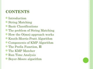
To find all occurrences of a pattern in a given text.
We can formalize the above statement by saying: Find a
given pattern p[1..m] in text
T[1..n] with n>=m.
Given a pattern P[1..m] and a text T[1..n], find all
occurrences of P in T. Both P and T belong to ∑*.
P occurs with shift s (beginning at s+1): P[1]=T[s+1],
P[2]=T[s+2],…,P[m]=T[s+m].
If so, call s is a valid shift, otherwise, an invalid shift.
Note: one occurrence begins within another one: P=abab,
T=abcabababbc, P occurs at s=3 and s=5.
*text is the string that we are searching.
*pattern is the string that we are searching for.
*Shift is an offset into a string.](https://image.slidesharecdn.com/stringmatchingalgorithm-150615142625-lva1-app6891/85/String-matching-algorithm-4-320.jpg)

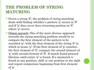
![Step 1:compare p[1] with S[1]
S
aa bb cc aa bb aa aa bb cc aa bb aa cc
p aa bb aa aa
Step 2: compare p[2] with S[2]
S aa bb cc aa bb aa aa bb cc aa bb aa cc
p aa bb aa aa](https://image.slidesharecdn.com/stringmatchingalgorithm-150615142625-lva1-app6891/85/String-matching-algorithm-8-320.jpg)
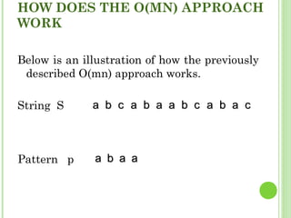
![Step 3: compare p[3] with S[3]
S
p aa bb aa aa
Mismatch occurs here..
Since mismatch is detected, shift ‘p’ one position to
the left and
perform steps analogous to those from step 1 to step
3. At position
where mismatch is detected, shift ‘p’ one position to
the right and
repeat matching procedure.
aa bb cc aa bb aa aa bb cc aa bb aa cc](https://image.slidesharecdn.com/stringmatchingalgorithm-150615142625-lva1-app6891/85/String-matching-algorithm-9-320.jpg)
![S aa bb cc aa bb aa aa bb cc aa bb aa cc
p aa bb aa aa
Finally, a match would be found after shifting ‘p’ three times to the right
side.
Drawbacks of this approach: if ‘m’ is the length of pattern ‘p’ and ‘n’ the
length of string ‘S’, the matching time is of the order O(mn). This is a
certainly a very slow running algorithm.
What makes this approach so slow is the fact that elements of ‘S’ with
which comparisons had been performed earlier are involved again and
again in comparisons in some future iterations. For example: when
mismatch is detected for the first time in comparison of p[3] with S[3],
pattern ‘p’ would be moved one position to the right and matching
procedure would resume from here. Here the first comparison that would
take place would be between p[0]=‘a’ and S[1]=‘b’. It should be noted here
that S[1]=‘b’ had been previously involved in a comparison in step 2. this is
a repetitive use of S[1] in another comparison. It is the repetitive
comparisons that lead to the runtime of O(mn).
#Knuth, Morris, and Pratt improved on this approach and found an](https://image.slidesharecdn.com/stringmatchingalgorithm-150615142625-lva1-app6891/85/String-matching-algorithm-10-320.jpg)

![THE PREFIX FUNCTION, Π
Following pseudo code computes the prefix
function, Π:
Compute-Prefix-Function (p)
1 m length[p] //’p’ pattern to be
matched
2 Π[1] 0
3 k 0
4 for q 2 to m
5 do while k > 0 and p[k+1] != p[q]
6 do k Π[k]
7 If p[k+1] = p[q]
8 then k k +1
9 Π[q] k
10 return Π](https://image.slidesharecdn.com/stringmatchingalgorithm-150615142625-lva1-app6891/85/String-matching-algorithm-13-320.jpg)
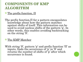
![Example: compute Π for the pattern ‘p’
below:
p aa bb aa bb aa cc aa
Initially: m = length[p] = 7
Π[1] = 0
k = 0
Step 1: q = 2, k=0
Π[2] = 0
Step 2: q = 3, k = 0,
Π[3] = 1
Step 3: q = 4, k = 1
Π[4] = 2
qq 11 22 33 44 55 66 77
pp aa bb aa bb aa cc aa
ΠΠ 00 00
qq 11 22 33 44 55 66 77
pp aa bb aa bb aa cc aa
ΠΠ 00 00 11
qq 11 22 33 44 55 66 77
pp aa bb aa bb aa cc AA
ΠΠ 00 00 11 22](https://image.slidesharecdn.com/stringmatchingalgorithm-150615142625-lva1-app6891/85/String-matching-algorithm-14-320.jpg)
![Step 4: q = 5, k =2
Π[5] = 3
Step 5: q = 6, k = 3
Π[6] = 1
Step 6: q = 7, k = 1
Π[7] = 1
After iterating 6 times, the
prefix function computation is
complete:
qq 11 22 33 44 55 66 77
pp aa bb aa bb aa cc aa
ΠΠ 00 00 11 22 33
qq 11 22 33 44 55 66 77
pp aa bb aa bb aa cc aa
ΠΠ 00 00 11 22 33 11
qq 11 22 33 44 55 66 77
pp aa bb aa bb aa cc aa
ΠΠ 00 00 11 22 33 11 11
qq 11 22 33 44 55 66 77
pp aa bb AA bb aa cc aa
ΠΠ 00 00 11 22 33 11 11](https://image.slidesharecdn.com/stringmatchingalgorithm-150615142625-lva1-app6891/85/String-matching-algorithm-15-320.jpg)
![THE KMP MATCHER
The KMP Matcher, with pattern ‘p’, string ‘S’ and prefix function ‘Π’ as input, finds a
match of p in S.
Following pseudo code computes the matching component of KMP algorithm:
KMP-Matcher(S,p)
1 n length[S]
2 m length[p]
3 Π Compute-Prefix-Function(p)
4 q 0 //number of characters matched
5 for i 1 to n //scan S from left to right
6 do while q > 0 and p[q+1] != S[i]
7 do q Π[q] //next character does not match
8 if p[q+1] = S[i]
9 then q q + 1 //next character matches
10 if q = m //is all of p matched?
11 then print “Pattern occurs with shift” i – m
12 q Π[ q] // look for the next match
Note: KMP finds every occurrence of a ‘p’ in ‘S’. That is why KMP does not terminate
in step 12, rather it searches remainder of ‘S’ for any more occurrences of ‘p’.](https://image.slidesharecdn.com/stringmatchingalgorithm-150615142625-lva1-app6891/85/String-matching-algorithm-16-320.jpg)
![bb aa cc bb aa bb aa bb aa bb aa cc aa aa bb
bb aa cc bb aa bb aa bb aa bb aa cc aa aa bb
aa bb aa bb aa cc aa
Initially: n = size of S = 15;
m = size of p = 7
Step 1: i = 1, q = 0
comparing p[1] with S[1]
S
p
P[1] does not match with S[1]. ‘p’ will be shifted one position to the right.
S
p aa bb aa bb aa cc aa
Step 2: i = 2, q = 0
comparing p[1] with S[2]
P[1] matches S[2]. Since there is a match, p is not shifted.](https://image.slidesharecdn.com/stringmatchingalgorithm-150615142625-lva1-app6891/85/String-matching-algorithm-18-320.jpg)
![Step 3: i = 3, q = 1
bb aa cc bb aa bb aa bb aa bb aa cc aa aa bb
Comparing p[2] with S[3]
S
aa bb aa bb aa cc aa
bb aa cc bb aa bb aa bb aa bb aa cc aa aa bb
bb aa cc bb aa bb aa bb aa bb aa cc aa aa bb
aa bb aa bb aa cc aa
aa bb aa bb aa cc aap
S
p
S
p
p[2] does not match with S[3]
Backtracking on p, comparing p[1] and S[3]
Step 4: i = 4, q = 0
comparing p[1] with S[4] p[1] does not match with S[4]
Step 5: i = 5, q = 0
comparing p[1] with S[5] p[1] matches with S[5]](https://image.slidesharecdn.com/stringmatchingalgorithm-150615142625-lva1-app6891/85/String-matching-algorithm-19-320.jpg)
![bb aa cc bb aa bb aa bb aa bb aa cc aa aa bb
bb aa cc bb aa bb aa bb aa bb aa cc aa aa bb
bb aa cc bb aa bb aa bb aa bb aa cc aa aa bb
aa bb aa bb aa cc aa
aa bb aa bb aa cc aa
aa bb aa bb aa cc aa
Step 6: i = 6, q = 1Step 6: i = 6, q = 1
S
p
Comparing p[2] with S[6] p[2] matches with S[6]
S
p
Step 7: i = 7, q = 2Step 7: i = 7, q = 2
Comparing p[3] with S[7] p[3] matches with S[7]
Step 8: i = 8, q = 3Step 8: i = 8, q = 3
Comparing p[4] with S[8] p[4] matches with S[8]
S
p](https://image.slidesharecdn.com/stringmatchingalgorithm-150615142625-lva1-app6891/85/String-matching-algorithm-20-320.jpg)
![Step 9: i = 9, q = 4Step 9: i = 9, q = 4
Comparing p[5] with S[9]
Comparing p[6] with S[10]
Comparing p[5] with S[11]
Step 10: i = 10, q = 5Step 10: i = 10, q = 5
Step 11: i = 11, q = 4Step 11: i = 11, q = 4
S
S
S
p
p
p
bb aa cc bb aa bb aa bb aa bb aa cc aa aa bb
bb aa cc bb aa bb aa bb aa bb aa cc aa aa bb
bb aa cc bb aa bb aa bb aa bb aa cc aa aa bb
aa bb aa bb aa cc aa
aa bb aa bb aa cc aa
aa bb aa bb aa cc aa
p[6] doesn’t match with S[10]
Backtracking on p, comparing p[4] with S[10] because after mismatch q = Π[5] = 3
p[5] matches with S[9]
p[5] matches with S[11]](https://image.slidesharecdn.com/stringmatchingalgorithm-150615142625-lva1-app6891/85/String-matching-algorithm-21-320.jpg)
![bb aa cc bb aa bb aa bb aa bb aa cc aa aa bb
bb aa cc bb aa bb aa bb aa bb aa cc aa aa bb
aa bb aa bb aa cc aa
aa bb aa bb aa cc aa
Step 12: i = 12, q = 5Step 12: i = 12, q = 5
Comparing p[6] with S[12]
Comparing p[7] with S[13]
S
S
p
p
Step 13: i = 13, q = 6Step 13: i = 13, q = 6
p[6] matches with S[12]
p[7] matches with S[13]
Pattern ‘p’ has been found to completely occur in string ‘S’. The total number of shifts
that took place for the match to be found are: i – m = 13 – 7 = 6 shifts.](https://image.slidesharecdn.com/stringmatchingalgorithm-150615142625-lva1-app6891/85/String-matching-algorithm-22-320.jpg)
![RUN TIME ANALYSIS
Compute-Prefix-Function (Π)
1 m length[p] //’p’ pattern to be
matched
2 Π[1] 0
3 k 0
4 for q 2 to m
5 do while k > 0 and p[k+1] != p[q]
6 do k Π[k]
7 If p[k+1] = p[q]
8 then k k +1
9 Π[q] k
10 return Π
In the above pseudocode for computing the
prefix function, the for loop from step 4
to step 10 runs ‘m’ times. Step 1 to
step 3 take constant time. Hence the
running time of compute prefix
function is Θ(m).
KMP Matcher
1 n length[S]
2 m length[p]
3 Π Compute-Prefix-Function(p)
4 q 0
5 for i 1 to n
6 do while q > 0 and p[q+1] != S[i]
7 do q Π[q]
8 if p[q+1] = S[i]
9 then q q + 1
10 if q = m
11 then print “Pattern occurs with shift” i
– m
12 q Π[ q]
The for loop beginning in step 5 runs ‘n’ times,
i.e., as long as the length of the string ‘S’.
Since step 1 to step 4 take constant time,
the running time is dominated by this for
loop. Thus running time of matching
function is Θ(n).](https://image.slidesharecdn.com/stringmatchingalgorithm-150615142625-lva1-app6891/85/String-matching-algorithm-23-320.jpg)


String matching algorithm
- 1. STRING MATCHING Alokeparna Choudhury(ME201310005) Stream. CSE Reg. No.2783 of 2009-10 University Institute of Technology
- 2. CONTENTS Introduction String Matching Basic Classifications The problem of String Matching How the O(mn) approach works Knuth-Morris-Pratt Algorithm Components of KMP Algorithm The Prefix Function, Π The KMP Matcher Run Time Analysis Boyer-Moore algorithm
- 3. INTRODUCTION o String matching algorithms, are an important class of string algorithms that try to find a place where one or several strings (also called patterns) are found within a larger string or text. Why do we need string matching? String matching is used in almost all the software applications straddling from simple text editors to the complex NIDS.
- 4. STRING MATCHING To find all occurrences of a pattern in a given text. We can formalize the above statement by saying: Find a given pattern p[1..m] in text T[1..n] with n>=m. Given a pattern P[1..m] and a text T[1..n], find all occurrences of P in T. Both P and T belong to ∑*. P occurs with shift s (beginning at s+1): P[1]=T[s+1], P[2]=T[s+2],…,P[m]=T[s+m]. If so, call s is a valid shift, otherwise, an invalid shift. Note: one occurrence begins within another one: P=abab, T=abcabababbc, P occurs at s=3 and s=5. *text is the string that we are searching. *pattern is the string that we are searching for. *Shift is an offset into a string.
- 5. BASIC CLASSIFICATION 1. Naïve algorithm: The naive approach for solving the string searching problem is accomplished by performing a Brute-Force comparison of each character in the pattern at each possible placement of the pattern in the string. This algorithm is O(mn) in the worst case. 2. Rabin – Karp algorithm: String matching algorithm that compares string’s hash values, rather than string themselves. Performs well in practice, and generalized to other algorithm for related problems, such as two- dimensional pattern matching. 3. Knuth-Morris-Pratt algorithm: It is improved on the Brute-force algorithm and the new algorithm is capable of running O(m+n) in the worst case. This algorithm improves the running time by taking advantage of tagged borders. 4. Boyer-Moore algorithm: The idea behind the Boyer-Moore algorithm is information gain. Here information is gained by beginning the comparison from the end of the pattern instead of the beginning. It performs the string searching task in sub linear time in the average case, which even KMP algorithm could not accomplish at that time.
- 6. THE PROBLEM OF STRING MATCHING Given a string ‘S’, the problem of string matching deals with finding whether a pattern ‘p’ occurs in ‘S’ and if ‘p’ does occur then returning position in ‘S’ where ‘p’ occurs. O(mn) aproach: One of the most obvious approach towards the string matching problem would be to compare the first element of the pattern to be searched ‘p’, with the first element of the string ‘S’ in which to locate ‘p’. If the first element of ‘p’ matches the first element of ‘S’, compare the second element of ‘p’ with second element of ‘S’. If match found proceed likewise until entire ‘p’ is found. If a mismatch is found at any position, shift ‘p’ one position to the right and repeat comparison beginning from first element of ‘p’.
- 7. HOW DOES THE O(MN) APPROACH WORK Below is an illustration of how the previously described O(mn) approach works. String S aa bb cc aa bb aa aa bb cc aa bb aa cc Pattern p aa bb aa aa
- 8. Step 1:compare p[1] with S[1] S aa bb cc aa bb aa aa bb cc aa bb aa cc p aa bb aa aa Step 2: compare p[2] with S[2] S aa bb cc aa bb aa aa bb cc aa bb aa cc p aa bb aa aa
- 9. Step 3: compare p[3] with S[3] S p aa bb aa aa Mismatch occurs here.. Since mismatch is detected, shift ‘p’ one position to the left and perform steps analogous to those from step 1 to step 3. At position where mismatch is detected, shift ‘p’ one position to the right and repeat matching procedure. aa bb cc aa bb aa aa bb cc aa bb aa cc
- 10. S aa bb cc aa bb aa aa bb cc aa bb aa cc p aa bb aa aa Finally, a match would be found after shifting ‘p’ three times to the right side. Drawbacks of this approach: if ‘m’ is the length of pattern ‘p’ and ‘n’ the length of string ‘S’, the matching time is of the order O(mn). This is a certainly a very slow running algorithm. What makes this approach so slow is the fact that elements of ‘S’ with which comparisons had been performed earlier are involved again and again in comparisons in some future iterations. For example: when mismatch is detected for the first time in comparison of p[3] with S[3], pattern ‘p’ would be moved one position to the right and matching procedure would resume from here. Here the first comparison that would take place would be between p[0]=‘a’ and S[1]=‘b’. It should be noted here that S[1]=‘b’ had been previously involved in a comparison in step 2. this is a repetitive use of S[1] in another comparison. It is the repetitive comparisons that lead to the runtime of O(mn). #Knuth, Morris, and Pratt improved on this approach and found an
- 11. KNUTH-MORRIS-PRATT ALGORITHM Knuth, Morris and Pratt proposed a linear time algorithm for the string matching problem. A matching time of O(n) is achieved by avoiding comparisons with elements of ‘S’ that have previously been involved in comparison with some element of the pattern ‘p’ to be matched. i.e., backtracking on the string ‘S’ never occurs.
- 12. COMPONENTS OF KMP ALGORITHM The prefix function, Π The prefix function,Π for a pattern encapsulates knowledge about how the pattern matches against shifts of itself. This information can be used to avoid useless shifts of the pattern ‘p’. In other words, this enables avoiding backtracking on the string ‘S’. The KMP Matcher With string ‘S’, pattern ‘p’ and prefix function ‘Π’ as inputs, finds the occurrence of ‘p’ in ‘S’ and returns the number of shifts of ‘p’ after which occurrence is found.
- 13. THE PREFIX FUNCTION, Π Following pseudo code computes the prefix function, Π: Compute-Prefix-Function (p) 1 m length[p] //’p’ pattern to be matched 2 Π[1] 0 3 k 0 4 for q 2 to m 5 do while k > 0 and p[k+1] != p[q] 6 do k Π[k] 7 If p[k+1] = p[q] 8 then k k +1 9 Π[q] k 10 return Π
- 14. Example: compute Π for the pattern ‘p’ below: p aa bb aa bb aa cc aa Initially: m = length[p] = 7 Π[1] = 0 k = 0 Step 1: q = 2, k=0 Π[2] = 0 Step 2: q = 3, k = 0, Π[3] = 1 Step 3: q = 4, k = 1 Π[4] = 2 qq 11 22 33 44 55 66 77 pp aa bb aa bb aa cc aa ΠΠ 00 00 qq 11 22 33 44 55 66 77 pp aa bb aa bb aa cc aa ΠΠ 00 00 11 qq 11 22 33 44 55 66 77 pp aa bb aa bb aa cc AA ΠΠ 00 00 11 22
- 15. Step 4: q = 5, k =2 Π[5] = 3 Step 5: q = 6, k = 3 Π[6] = 1 Step 6: q = 7, k = 1 Π[7] = 1 After iterating 6 times, the prefix function computation is complete: qq 11 22 33 44 55 66 77 pp aa bb aa bb aa cc aa ΠΠ 00 00 11 22 33 qq 11 22 33 44 55 66 77 pp aa bb aa bb aa cc aa ΠΠ 00 00 11 22 33 11 qq 11 22 33 44 55 66 77 pp aa bb aa bb aa cc aa ΠΠ 00 00 11 22 33 11 11 qq 11 22 33 44 55 66 77 pp aa bb AA bb aa cc aa ΠΠ 00 00 11 22 33 11 11
- 16. THE KMP MATCHER The KMP Matcher, with pattern ‘p’, string ‘S’ and prefix function ‘Π’ as input, finds a match of p in S. Following pseudo code computes the matching component of KMP algorithm: KMP-Matcher(S,p) 1 n length[S] 2 m length[p] 3 Π Compute-Prefix-Function(p) 4 q 0 //number of characters matched 5 for i 1 to n //scan S from left to right 6 do while q > 0 and p[q+1] != S[i] 7 do q Π[q] //next character does not match 8 if p[q+1] = S[i] 9 then q q + 1 //next character matches 10 if q = m //is all of p matched? 11 then print “Pattern occurs with shift” i – m 12 q Π[ q] // look for the next match Note: KMP finds every occurrence of a ‘p’ in ‘S’. That is why KMP does not terminate in step 12, rather it searches remainder of ‘S’ for any more occurrences of ‘p’.
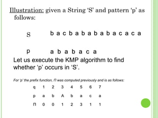
- 17. Illustration: given a String ‘S’ and pattern ‘p’ as follows: S bb aa cc bb aa bb aa bb aa bb aa cc aa cc aa p aa bb aa bb aa cc aa Let us execute the KMP algorithm to find whether ‘p’ occurs in ‘S’. For ‘p’ the prefix function, Π was computed previously and is as follows: qq 11 22 33 44 55 66 77 pp aa bb AA bb aa cc aa ΠΠ 00 00 11 22 33 11 11
- 18. bb aa cc bb aa bb aa bb aa bb aa cc aa aa bb bb aa cc bb aa bb aa bb aa bb aa cc aa aa bb aa bb aa bb aa cc aa Initially: n = size of S = 15; m = size of p = 7 Step 1: i = 1, q = 0 comparing p[1] with S[1] S p P[1] does not match with S[1]. ‘p’ will be shifted one position to the right. S p aa bb aa bb aa cc aa Step 2: i = 2, q = 0 comparing p[1] with S[2] P[1] matches S[2]. Since there is a match, p is not shifted.
- 19. Step 3: i = 3, q = 1 bb aa cc bb aa bb aa bb aa bb aa cc aa aa bb Comparing p[2] with S[3] S aa bb aa bb aa cc aa bb aa cc bb aa bb aa bb aa bb aa cc aa aa bb bb aa cc bb aa bb aa bb aa bb aa cc aa aa bb aa bb aa bb aa cc aa aa bb aa bb aa cc aap S p S p p[2] does not match with S[3] Backtracking on p, comparing p[1] and S[3] Step 4: i = 4, q = 0 comparing p[1] with S[4] p[1] does not match with S[4] Step 5: i = 5, q = 0 comparing p[1] with S[5] p[1] matches with S[5]
- 20. bb aa cc bb aa bb aa bb aa bb aa cc aa aa bb bb aa cc bb aa bb aa bb aa bb aa cc aa aa bb bb aa cc bb aa bb aa bb aa bb aa cc aa aa bb aa bb aa bb aa cc aa aa bb aa bb aa cc aa aa bb aa bb aa cc aa Step 6: i = 6, q = 1Step 6: i = 6, q = 1 S p Comparing p[2] with S[6] p[2] matches with S[6] S p Step 7: i = 7, q = 2Step 7: i = 7, q = 2 Comparing p[3] with S[7] p[3] matches with S[7] Step 8: i = 8, q = 3Step 8: i = 8, q = 3 Comparing p[4] with S[8] p[4] matches with S[8] S p
- 21. Step 9: i = 9, q = 4Step 9: i = 9, q = 4 Comparing p[5] with S[9] Comparing p[6] with S[10] Comparing p[5] with S[11] Step 10: i = 10, q = 5Step 10: i = 10, q = 5 Step 11: i = 11, q = 4Step 11: i = 11, q = 4 S S S p p p bb aa cc bb aa bb aa bb aa bb aa cc aa aa bb bb aa cc bb aa bb aa bb aa bb aa cc aa aa bb bb aa cc bb aa bb aa bb aa bb aa cc aa aa bb aa bb aa bb aa cc aa aa bb aa bb aa cc aa aa bb aa bb aa cc aa p[6] doesn’t match with S[10] Backtracking on p, comparing p[4] with S[10] because after mismatch q = Π[5] = 3 p[5] matches with S[9] p[5] matches with S[11]
- 22. bb aa cc bb aa bb aa bb aa bb aa cc aa aa bb bb aa cc bb aa bb aa bb aa bb aa cc aa aa bb aa bb aa bb aa cc aa aa bb aa bb aa cc aa Step 12: i = 12, q = 5Step 12: i = 12, q = 5 Comparing p[6] with S[12] Comparing p[7] with S[13] S S p p Step 13: i = 13, q = 6Step 13: i = 13, q = 6 p[6] matches with S[12] p[7] matches with S[13] Pattern ‘p’ has been found to completely occur in string ‘S’. The total number of shifts that took place for the match to be found are: i – m = 13 – 7 = 6 shifts.
- 23. RUN TIME ANALYSIS Compute-Prefix-Function (Π) 1 m length[p] //’p’ pattern to be matched 2 Π[1] 0 3 k 0 4 for q 2 to m 5 do while k > 0 and p[k+1] != p[q] 6 do k Π[k] 7 If p[k+1] = p[q] 8 then k k +1 9 Π[q] k 10 return Π In the above pseudocode for computing the prefix function, the for loop from step 4 to step 10 runs ‘m’ times. Step 1 to step 3 take constant time. Hence the running time of compute prefix function is Θ(m). KMP Matcher 1 n length[S] 2 m length[p] 3 Π Compute-Prefix-Function(p) 4 q 0 5 for i 1 to n 6 do while q > 0 and p[q+1] != S[i] 7 do q Π[q] 8 if p[q+1] = S[i] 9 then q q + 1 10 if q = m 11 then print “Pattern occurs with shift” i – m 12 q Π[ q] The for loop beginning in step 5 runs ‘n’ times, i.e., as long as the length of the string ‘S’. Since step 1 to step 4 take constant time, the running time is dominated by this for loop. Thus running time of matching function is Θ(n).
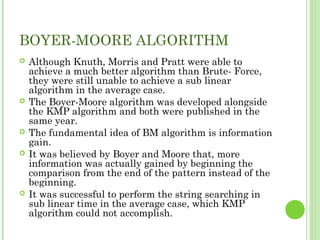
- 24. BOYER-MOORE ALGORITHM Although Knuth, Morris and Pratt were able to achieve a much better algorithm than Brute- Force, they were still unable to achieve a sub linear algorithm in the average case. The Boyer-Moore algorithm was developed alongside the KMP algorithm and both were published in the same year. The fundamental idea of BM algorithm is information gain. It was believed by Boyer and Moore that, more information was actually gained by beginning the comparison from the end of the pattern instead of the beginning. It was successful to perform the string searching in sub linear time in the average case, which KMP algorithm could not accomplish.
- 25. WHAT IS IT ABOUT? A String Matching Algorithm Preprocess a Pattern P (|P| = n) For a text T (| T| = m), find all of the occurrences of P in T Time complexity: O(n + m), but usually sub-linear, O(n/m) The worst case of BM algorithm could be O(nm) or O(n+m) based on the heuristics used.
- 26. THANK YOU