SlideShare a Scribd company logo
Things and Analytics
Supervised Learning
• Two types of data samples
• Training: Used to extract
features and train the
machine learning algorithm
• Testing: Used to predict the
label for the given test data
• Supervised learning can be
used for both classification
and regression tasks
Contd..
• Classification: To
separate into
classes
• Regression: To
predict the
dependent variable
a.) Classification
b.) Regression
k- Nearest Neighbors
• Based on majority voting
among nearest neighbors,
the sample is classified into
the majority class.
• Consider the example on
the right
• Classify the point
<Temperature = 4 and
Humidity = 8> with = 3.
Temperature Humidity Class
a 8 8 Warm
b 8 5 Warm
c 4 5 Cool
d 2 5 Cool
e 9 9 Warm
Contd..
• Denote the test sample as x.
• Using Euclidean measure:
• D(x, a) =
• D(x, b) =
• D(x, c) =
• D(x, d) =
• D(x, e) =
• Clearly c, d and a are the nearest neighbors of x. Majority of
the nearest neighbors (2 out of 3) fall in the Cool class.
Therefore, x is Cool.
Naïve Bayes Classification
• Conditional probability
Contd..
• Consider the example given.
• P(Sunny) = 3/12
• P(Rainy) = 4/12
• P(Windy) = 5/12
• P (No) = 3/12
• P(Yes) = 9/12
• Find P(Yes|Windy)
• P (Windy|Yes) = 3/9 (In 9 Yes,
there are 3 Windy)
•
Weather No Yes Probability
Sunny 1 2
Rainy 0 4
Windy 2 3
Probabilit
y
Linear Regression
• The equation of a line
• y = ax + b
• Calculate b as
• Calculate a as
= days 1 2 4 6 7
= productivity 2 3 5 4 10
Linear Regression
• = 0.8
• If x = 8, y = 8.8. = days 1 2 4 6 7
= productivity 2 3 5 4 10
Limitations of Linear Regression
• Linear regression gives a numerical result
• Logistic regression gives an output between 0 and 1
• If the output is greater than some threshold, say, 0.5, the logistic
regression gives 1, otherwise 0
Logistic Regression
• Define z
• Logistic regression defines probability as:
Contd..
• Assume that the hypothesis
for linear regression is
• Ques. 1. Determine the
probability of having a
disease who has glucose
level 30.
•
Glucose level Result
18 0
16 0
32 1
27 1
40 1
Contd..
• Assume that the hypothesis for linear
regression is
• Ques. 2. What glucose level ensures
a probability of more than 98%?
•
• = 0.020408
• z = 3.891828
• Putting z in
• Glucose Level = 29.945914.
Glucose level Result
18 0
16 0
32 1
27 1
40 1
Unsupervised Learning
• In unsupervised learning, given
data samples, we group similar
data together
• Data samples are clustered
based on similarity
Flowchart of Unsupervised
Learning
Clustering
Principal Component Analysis
• Unsupervised learning technique for dimensionality
reduction in N-dimensional datasets
• Reduced dimensionality eliminates redundancy
• Keep maximum variance among reduced axis
• Before applying PCA, we make the data set having zero
mean using the centering technique
Contd..
• Find the first principal
component of the data in
Table 6.5
• Note that
•
• Table 6.6 gives important
parameters
2.4375
= Soil Moisture 2 1 0 -1
= Leaf Wetness 4 3 1 0.5
Smart agriculture data for PCA problem
Contd..
• (By taking values from Table 6.6)
• Similarly,
• Similarly
Contd..
• S = =
• Put
• = 0
• Solving this equation (using calculator or online tool), you will get
roots as 4.35 and 0.052.
1.67 2.08
2.08 2.73
Contd..
• Considering the largest eigenvalue, we get the first principal
component from the eigen-vector direction.
• Get eigenvector as:
• Solve
•
Contd..
•
• Now, 2D data is reduced to 1D data in the direction of the
principal component.
• Therefore, transforming the data into new subspace as:
Bias and Variance Tradeoff
• Underfitting
• The data is modelled by an order lower
than the actual order of the model.
• High bias condition
• Overfitting
• The data is modelled by an order
higher than the actual order of the
model.
• High variance condition
• The model memorizes the training data
• If we apply unseen test data to this
overfitted model, the error is high.
Contd..
• The data on the right shows a
quadratic model
• If we plot the data using these
three plots:
• The RMSE is 1.724, 0.3696, 0.3227
for the first, second, and the third
order models respectively
• Even though the RMSE is least for the
third order model, it is an overfitted
model.
Data
and its
scatter
plot!
0 1 2 3 4
0 1 4.8 9.4 15.5
Artificial Neural Networks
• Take inspiration from neurons in human
brain
• Dendrites are the thin fiber that carries
information from other neurons.
• The information transmitted between the
dendrites and axons is carried out by the
synapse
• This information is then passed to the cell
body for processing.
• Axon carries impulses from the cell body to
other cells.
• Dendrites, synapse, cell body (or soma),
and axon of a biological neuron
correspond to input, weight, node, and
output of an artificial neuron,
respectively
• We get the output if the sum of weighted
information is greater than a threshold.
Perceptron Model
• A single unit of neuron
• The output is unity if the
weighted sum of the input is
greater than zero.
• For example:
• If , , , , , and , the weighted sum of
inputs is 7 and hence the output is
1. On the other hand, if , , , , , and ,
the weighted sum of inputs is -1
and hence the output is 0.
Activation Function
• Activation function decides whether a neuron will be
activated or not
• Activation function helps us to introduce non-linearity which
is helpful in learning complex models
• There are many different activation functions discussed in
literature
Linear and Binary Step Activation
Functions
h(𝑥)=𝑥
Sigmoid and Tanh Activation Functions
h(𝑥)=
1
1+𝑒
−𝑥 h(𝑥)=
𝑒𝑥
−𝑒−𝑥
𝑒
𝑥
+𝑒
−𝑥
Tanh activation function is also known as
Bipolar Sigmoid activation function
ReLU Activation Function
• Most used.
• Efficient
Loss Functions
• The objective in training neural networks is to minimize the loss function.
Different loss functions are:
• Mean Absolute Error (MAE)
• Here, is the predicted value and is the true value
• Mean Squared Error (MSE)
• Cross-Entropy (CE) Loss
• Used in Classification problems
• Here p is the true distribution, and q is the estimated distribution
• Here, is the Kullback-Leibler divergence between the two distributions
Back-propagation
• Backpropagation is used to train neural networks
• Compute the gradient of a cost function with respect to all the
weights in the network and backpropagate error (loss) information
• Consider the example:
Contd…
• Solution
• Similarly,
• Subsequently, the loss is computed using the mean squared error
as
• [desired is assumed to be 1]
Contd…
• Solution
• This error must be backpropagated through the neural network
• First, we calculate
• Denote, , then
• So,
• Then,
• And
Contd…
• Solution
• Denote
• Also,
• Using chain rule for derivatives, we have:
• Assume the learning rate
• Update
• Similarly, calculate for
Optimization in Back-Propagation
• Gradient Descent Method
• First derivative of a scalar function E(w) with respect to a vector w =
[w1, w2]T
is called the gradient of E(w) or
• The second derivative of a scalar function E(w) with respect to a
vector is a matrix called the Hessian of or
Contd…
• Batch gradient descent
• Computes the gradient of the cost function with respect to the
parameters w for the entire training dataset
• For a function , derivative (slope at point w) of it is
• A small change () in the input can cause the output to move to a
value given by [via first order Taylor series]
• Assuming minimization, we take a jump such that y reduces
• Gradient descent proposes weight update as
• Here is the learning rate and m is the batch-size
Contd…
• Batch Gradient Descent (Example):
• Let there be 100 samples in a dataset that are used for training the
model
• For batch gradient descent, batch size = 100 and there is only 1 batch
• The updated weight w’ is obtained by summing the gradients of all
losses considering all samples and then averaging them
• Here,
Contd…
• Batch Gradient Descent (Example):
• If there are 6 examples in the dataset,
• Let the target values corresponding to examples be respectively
• Let the weights associated with these examples are
• Let the derivative of loss for be 0.5, 0.2, 0.7, 0.4, 0.7, and 0.6 respectively
initially.
• Using gradient descent, we update weight as follows:
• Since, and let
• Similarly, all weights are updated until convergence or maximum
number of allowed iterations
Contd…
• Minibatch gradient descent
• Perform update for every mini-batch of n examples.
• The weight is updated as:
• Here, is the learning rate and . Mini-batch size is a hyperparameter
Contd…
• Mini-batch gradient descent (Example):
• Let there be 100 samples
• Mini-batches = 5, Batch-size = 20
• Updated weight w’ is obtained by summing the gradients of losses
considering 20 samples and then averaging them
• Here,
• Update weight for each mini-batch till convergence or maximum
number of allowed iterations
Contd…
• Mini-batch gradient descent (Example):
• Consider the same example as Batch Gradient Descent
• Consider 2 mini-batches with batch-size of 3
• Using minibatch gradient descent, is updates as:
•
• Similarly, all weights are updated until convergence or maximum
number of allowed iterations
Contd…
• Stochastic Gradient Descent
• In stochastic gradient descent, a single parameter update takes
place
• It is fast as it avoids redundancy that exists in batch gradient
descent
• It performs frequent updates with a high variance that causes the
objective function to fluctuate heavily
Contd…
• Stochastic gradient descent (Example):
• Consider 100 samples in a dataset
• Batch size = 1, Number of batches = 100
• Updated weight w’ is obtained by summing the gradients of loss of
each sample at a time
• Here,
• The weight is updated for every single sample
• The oscillation is very high compared to gradient descent before reaching
global optima
Contd…
• Stochastic gradient descent (Example):
• Consider the same example as Batch Gradient Descent
• Using SGD, we update weight as follows
• Here, ,
• SGD is faster when compared with GD
• However, weight update oscillates with SGD
• GD updates convergence without much oscillations
Evaluation Methods
• Dataset is divided into train and test sets
• Train set
• Used for model training
• Test set
• Disjoint from training set
• Also called holdout set
• Validation set (sometimes a 3-way split)
• Sometimes test set is held out to give only the final answer
• In that case, validation set can be used as an intermediary test set
• An example of overfitting is when the training loss decreases but the
validation loss increases
Contd..
• n-fold Cross-validation
• If we are running the algorithm for n times, and using the same test data,
chances are that overfitting will occur
• Instead, we divide the dataset into n parts. We use each part as a test set in different
iteration and the remaining (n-1) parts combined as the training set
• In this way, we have a new test set every iteration, and the dataset size is the same
• The procedure runs n times and gives n accuracies. The final accuracy is the average of
the n accuracies
• Leave-one-out Cross-validation
• This method is used when the dataset is very small
• Each fold of the cross-validation has only a single test example. The rest of
the data is used for training
• If the original data has m-examples, we can run the procedure over m-iterations and get
the average
Performance Metrics
• Accuracy
• Ratio of the number of correctly predicted
results to the total number of predicted results
• Precision
• Number of correctly classified positive examples
divided by the total number of examples that
are classified as positive
• Recall
• Number of correctly classified positive examples
divided by the total number of actual positive
examples in the test set
• F1 Score
• Combination of precision and recall into one
measure
•
• If FP = FN = 0, then F1 Score = 1
Confusion Matrix
Contd..
• If TP = 1, TN = 1000, FP = 0, and FN = 99, then from
equations before, we get: accuracy = 91 %, precision p =
100%, recall r =1%.
• F1 Score =
• Note
• F1-score is a harmonic mean
• F1-score tends to be closer to the smaller of the two: precision and recall
• Useful to determine the worst performance of the two

More Related Content

Similar to Supervised learning for IOT IN Vellore Institute of Technology (20)

PDF
Logistic regression
MartinHogg9
 
PDF
Lecture 4 - Linear Regression, a lecture in subject module Statistical & Mach...
Maninda Edirisooriya
 
PPTX
regression analysis presentation slides.
nsnatraj23
 
PPTX
Reason To Switch to DNNDNNs excel in handling huge volumes of data (e.g., ima...
SrideviPcSenthilkuma
 
PPTX
Nimrita deep learning
Nimrita Koul
 
PPTX
crossvalidation.pptx
PriyadharshiniG41
 
PPTX
Regression ppt
SuyashSingh70
 
PDF
Linear regression
MartinHogg9
 
PDF
Artificial Intelligence Course: Linear models
ananth
 
PPTX
Techniques in Deep Learning
Sourya Dey
 
PDF
ARTIFICIAL-NEURAL-NETWORKMACHINELEARNING
mohanapriyastp
 
PDF
L1 intro2 supervised_learning
Yogendra Singh
 
PPTX
08 neural networks
ankit_ppt
 
PPTX
Introduction to Deep Learning
Mehrnaz Faraz
 
PPTX
An Introduction to Deep Learning
milad abbasi
 
PPTX
Deep Learning Interview Questions And Answers | AI & Deep Learning Interview ...
Simplilearn
 
PDF
Model Selection and Validation
gmorishita
 
PPTX
ngboost.pptx
Hadrian7
 
PPTX
Build_Machine_Learning_System for Machine Learning Course
ssuserfece35
 
PPTX
Optimization techniq
RakshithGowdakodihal
 
Logistic regression
MartinHogg9
 
Lecture 4 - Linear Regression, a lecture in subject module Statistical & Mach...
Maninda Edirisooriya
 
regression analysis presentation slides.
nsnatraj23
 
Reason To Switch to DNNDNNs excel in handling huge volumes of data (e.g., ima...
SrideviPcSenthilkuma
 
Nimrita deep learning
Nimrita Koul
 
crossvalidation.pptx
PriyadharshiniG41
 
Regression ppt
SuyashSingh70
 
Linear regression
MartinHogg9
 
Artificial Intelligence Course: Linear models
ananth
 
Techniques in Deep Learning
Sourya Dey
 
ARTIFICIAL-NEURAL-NETWORKMACHINELEARNING
mohanapriyastp
 
L1 intro2 supervised_learning
Yogendra Singh
 
08 neural networks
ankit_ppt
 
Introduction to Deep Learning
Mehrnaz Faraz
 
An Introduction to Deep Learning
milad abbasi
 
Deep Learning Interview Questions And Answers | AI & Deep Learning Interview ...
Simplilearn
 
Model Selection and Validation
gmorishita
 
ngboost.pptx
Hadrian7
 
Build_Machine_Learning_System for Machine Learning Course
ssuserfece35
 
Optimization techniq
RakshithGowdakodihal
 

Recently uploaded (20)

PDF
Pressure Measurement training for engineers and Technicians
AIESOLUTIONS
 
PPTX
Hashing Introduction , hash functions and techniques
sailajam21
 
PPTX
美国电子版毕业证南卡罗莱纳大学上州分校水印成绩单USC学费发票定做学位证书编号怎么查
Taqyea
 
PPTX
原版一样(Acadia毕业证书)加拿大阿卡迪亚大学毕业证办理方法
Taqyea
 
PPTX
MobileComputingMANET2023 MobileComputingMANET2023.pptx
masterfake98765
 
PPTX
artificial intelligence applications in Geomatics
NawrasShatnawi1
 
PDF
GTU Civil Engineering All Semester Syllabus.pdf
Vimal Bhojani
 
PPTX
Lecture 1 Shell and Tube Heat exchanger-1.pptx
mailforillegalwork
 
PDF
Water Industry Process Automation & Control Monthly July 2025
Water Industry Process Automation & Control
 
PPTX
Day2 B2 Best.pptx
helenjenefa1
 
PPTX
Element 7. CHEMICAL AND BIOLOGICAL AGENT.pptx
merrandomohandas
 
PPTX
Element 11. ELECTRICITY safety and hazards
merrandomohandas
 
PPT
Carmon_Remote Sensing GIS by Mahesh kumar
DhananjayM6
 
PPTX
DATA BASE MANAGEMENT AND RELATIONAL DATA
gomathisankariv2
 
PDF
MAD Unit - 1 Introduction of Android IT Department
JappanMavani
 
DOCX
CS-802 (A) BDH Lab manual IPS Academy Indore
thegodhimself05
 
PPTX
What is Shot Peening | Shot Peening is a Surface Treatment Process
Vibra Finish
 
PPTX
Green Building & Energy Conservation ppt
Sagar Sarangi
 
PDF
Biomechanics of Gait: Engineering Solutions for Rehabilitation (www.kiu.ac.ug)
publication11
 
PPTX
Heart Bleed Bug - A case study (Course: Cryptography and Network Security)
Adri Jovin
 
Pressure Measurement training for engineers and Technicians
AIESOLUTIONS
 
Hashing Introduction , hash functions and techniques
sailajam21
 
美国电子版毕业证南卡罗莱纳大学上州分校水印成绩单USC学费发票定做学位证书编号怎么查
Taqyea
 
原版一样(Acadia毕业证书)加拿大阿卡迪亚大学毕业证办理方法
Taqyea
 
MobileComputingMANET2023 MobileComputingMANET2023.pptx
masterfake98765
 
artificial intelligence applications in Geomatics
NawrasShatnawi1
 
GTU Civil Engineering All Semester Syllabus.pdf
Vimal Bhojani
 
Lecture 1 Shell and Tube Heat exchanger-1.pptx
mailforillegalwork
 
Water Industry Process Automation & Control Monthly July 2025
Water Industry Process Automation & Control
 
Day2 B2 Best.pptx
helenjenefa1
 
Element 7. CHEMICAL AND BIOLOGICAL AGENT.pptx
merrandomohandas
 
Element 11. ELECTRICITY safety and hazards
merrandomohandas
 
Carmon_Remote Sensing GIS by Mahesh kumar
DhananjayM6
 
DATA BASE MANAGEMENT AND RELATIONAL DATA
gomathisankariv2
 
MAD Unit - 1 Introduction of Android IT Department
JappanMavani
 
CS-802 (A) BDH Lab manual IPS Academy Indore
thegodhimself05
 
What is Shot Peening | Shot Peening is a Surface Treatment Process
Vibra Finish
 
Green Building & Energy Conservation ppt
Sagar Sarangi
 
Biomechanics of Gait: Engineering Solutions for Rehabilitation (www.kiu.ac.ug)
publication11
 
Heart Bleed Bug - A case study (Course: Cryptography and Network Security)
Adri Jovin
 
Ad

Supervised learning for IOT IN Vellore Institute of Technology

  • 2. Supervised Learning • Two types of data samples • Training: Used to extract features and train the machine learning algorithm • Testing: Used to predict the label for the given test data • Supervised learning can be used for both classification and regression tasks
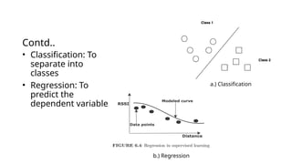
  • 3. Contd.. • Classification: To separate into classes • Regression: To predict the dependent variable a.) Classification b.) Regression
  • 4. k- Nearest Neighbors • Based on majority voting among nearest neighbors, the sample is classified into the majority class. • Consider the example on the right • Classify the point <Temperature = 4 and Humidity = 8> with = 3. Temperature Humidity Class a 8 8 Warm b 8 5 Warm c 4 5 Cool d 2 5 Cool e 9 9 Warm
  • 5. Contd.. • Denote the test sample as x. • Using Euclidean measure: • D(x, a) = • D(x, b) = • D(x, c) = • D(x, d) = • D(x, e) = • Clearly c, d and a are the nearest neighbors of x. Majority of the nearest neighbors (2 out of 3) fall in the Cool class. Therefore, x is Cool.
  • 6. Naïve Bayes Classification • Conditional probability
  • 7. Contd.. • Consider the example given. • P(Sunny) = 3/12 • P(Rainy) = 4/12 • P(Windy) = 5/12 • P (No) = 3/12 • P(Yes) = 9/12 • Find P(Yes|Windy) • P (Windy|Yes) = 3/9 (In 9 Yes, there are 3 Windy) • Weather No Yes Probability Sunny 1 2 Rainy 0 4 Windy 2 3 Probabilit y
  • 8. Linear Regression • The equation of a line • y = ax + b • Calculate b as • Calculate a as = days 1 2 4 6 7 = productivity 2 3 5 4 10
  • 9. Linear Regression • = 0.8 • If x = 8, y = 8.8. = days 1 2 4 6 7 = productivity 2 3 5 4 10
  • 10. Limitations of Linear Regression • Linear regression gives a numerical result • Logistic regression gives an output between 0 and 1 • If the output is greater than some threshold, say, 0.5, the logistic regression gives 1, otherwise 0
  • 11. Logistic Regression • Define z • Logistic regression defines probability as:
  • 12. Contd.. • Assume that the hypothesis for linear regression is • Ques. 1. Determine the probability of having a disease who has glucose level 30. • Glucose level Result 18 0 16 0 32 1 27 1 40 1
  • 13. Contd.. • Assume that the hypothesis for linear regression is • Ques. 2. What glucose level ensures a probability of more than 98%? • • = 0.020408 • z = 3.891828 • Putting z in • Glucose Level = 29.945914. Glucose level Result 18 0 16 0 32 1 27 1 40 1
  • 14. Unsupervised Learning • In unsupervised learning, given data samples, we group similar data together • Data samples are clustered based on similarity Flowchart of Unsupervised Learning Clustering
  • 15. Principal Component Analysis • Unsupervised learning technique for dimensionality reduction in N-dimensional datasets • Reduced dimensionality eliminates redundancy • Keep maximum variance among reduced axis • Before applying PCA, we make the data set having zero mean using the centering technique
  • 16. Contd.. • Find the first principal component of the data in Table 6.5 • Note that • • Table 6.6 gives important parameters 2.4375 = Soil Moisture 2 1 0 -1 = Leaf Wetness 4 3 1 0.5 Smart agriculture data for PCA problem
  • 17. Contd.. • (By taking values from Table 6.6) • Similarly, • Similarly
  • 18. Contd.. • S = = • Put • = 0 • Solving this equation (using calculator or online tool), you will get roots as 4.35 and 0.052. 1.67 2.08 2.08 2.73
  • 19. Contd.. • Considering the largest eigenvalue, we get the first principal component from the eigen-vector direction. • Get eigenvector as: • Solve •
  • 20. Contd.. • • Now, 2D data is reduced to 1D data in the direction of the principal component. • Therefore, transforming the data into new subspace as:
  • 21. Bias and Variance Tradeoff • Underfitting • The data is modelled by an order lower than the actual order of the model. • High bias condition • Overfitting • The data is modelled by an order higher than the actual order of the model. • High variance condition • The model memorizes the training data • If we apply unseen test data to this overfitted model, the error is high.
  • 22. Contd.. • The data on the right shows a quadratic model • If we plot the data using these three plots: • The RMSE is 1.724, 0.3696, 0.3227 for the first, second, and the third order models respectively • Even though the RMSE is least for the third order model, it is an overfitted model. Data and its scatter plot! 0 1 2 3 4 0 1 4.8 9.4 15.5
  • 23. Artificial Neural Networks • Take inspiration from neurons in human brain • Dendrites are the thin fiber that carries information from other neurons. • The information transmitted between the dendrites and axons is carried out by the synapse • This information is then passed to the cell body for processing. • Axon carries impulses from the cell body to other cells. • Dendrites, synapse, cell body (or soma), and axon of a biological neuron correspond to input, weight, node, and output of an artificial neuron, respectively • We get the output if the sum of weighted information is greater than a threshold.
  • 24. Perceptron Model • A single unit of neuron • The output is unity if the weighted sum of the input is greater than zero. • For example: • If , , , , , and , the weighted sum of inputs is 7 and hence the output is 1. On the other hand, if , , , , , and , the weighted sum of inputs is -1 and hence the output is 0.
  • 25. Activation Function • Activation function decides whether a neuron will be activated or not • Activation function helps us to introduce non-linearity which is helpful in learning complex models • There are many different activation functions discussed in literature
  • 26. Linear and Binary Step Activation Functions h(𝑥)=𝑥
  • 27. Sigmoid and Tanh Activation Functions h(𝑥)= 1 1+𝑒 −𝑥 h(𝑥)= 𝑒𝑥 −𝑒−𝑥 𝑒 𝑥 +𝑒 −𝑥 Tanh activation function is also known as Bipolar Sigmoid activation function
  • 28. ReLU Activation Function • Most used. • Efficient
  • 29. Loss Functions • The objective in training neural networks is to minimize the loss function. Different loss functions are: • Mean Absolute Error (MAE) • Here, is the predicted value and is the true value • Mean Squared Error (MSE) • Cross-Entropy (CE) Loss • Used in Classification problems • Here p is the true distribution, and q is the estimated distribution • Here, is the Kullback-Leibler divergence between the two distributions
  • 30. Back-propagation • Backpropagation is used to train neural networks • Compute the gradient of a cost function with respect to all the weights in the network and backpropagate error (loss) information • Consider the example:
  • 31. Contd… • Solution • Similarly, • Subsequently, the loss is computed using the mean squared error as • [desired is assumed to be 1]
  • 32. Contd… • Solution • This error must be backpropagated through the neural network • First, we calculate • Denote, , then • So, • Then, • And
  • 33. Contd… • Solution • Denote • Also, • Using chain rule for derivatives, we have: • Assume the learning rate • Update • Similarly, calculate for
  • 34. Optimization in Back-Propagation • Gradient Descent Method • First derivative of a scalar function E(w) with respect to a vector w = [w1, w2]T is called the gradient of E(w) or • The second derivative of a scalar function E(w) with respect to a vector is a matrix called the Hessian of or
  • 35. Contd… • Batch gradient descent • Computes the gradient of the cost function with respect to the parameters w for the entire training dataset • For a function , derivative (slope at point w) of it is • A small change () in the input can cause the output to move to a value given by [via first order Taylor series] • Assuming minimization, we take a jump such that y reduces • Gradient descent proposes weight update as • Here is the learning rate and m is the batch-size
  • 36. Contd… • Batch Gradient Descent (Example): • Let there be 100 samples in a dataset that are used for training the model • For batch gradient descent, batch size = 100 and there is only 1 batch • The updated weight w’ is obtained by summing the gradients of all losses considering all samples and then averaging them • Here,
  • 37. Contd… • Batch Gradient Descent (Example): • If there are 6 examples in the dataset, • Let the target values corresponding to examples be respectively • Let the weights associated with these examples are • Let the derivative of loss for be 0.5, 0.2, 0.7, 0.4, 0.7, and 0.6 respectively initially. • Using gradient descent, we update weight as follows: • Since, and let • Similarly, all weights are updated until convergence or maximum number of allowed iterations
  • 38. Contd… • Minibatch gradient descent • Perform update for every mini-batch of n examples. • The weight is updated as: • Here, is the learning rate and . Mini-batch size is a hyperparameter
  • 39. Contd… • Mini-batch gradient descent (Example): • Let there be 100 samples • Mini-batches = 5, Batch-size = 20 • Updated weight w’ is obtained by summing the gradients of losses considering 20 samples and then averaging them • Here, • Update weight for each mini-batch till convergence or maximum number of allowed iterations
  • 40. Contd… • Mini-batch gradient descent (Example): • Consider the same example as Batch Gradient Descent • Consider 2 mini-batches with batch-size of 3 • Using minibatch gradient descent, is updates as: • • Similarly, all weights are updated until convergence or maximum number of allowed iterations
  • 41. Contd… • Stochastic Gradient Descent • In stochastic gradient descent, a single parameter update takes place • It is fast as it avoids redundancy that exists in batch gradient descent • It performs frequent updates with a high variance that causes the objective function to fluctuate heavily
  • 42. Contd… • Stochastic gradient descent (Example): • Consider 100 samples in a dataset • Batch size = 1, Number of batches = 100 • Updated weight w’ is obtained by summing the gradients of loss of each sample at a time • Here, • The weight is updated for every single sample • The oscillation is very high compared to gradient descent before reaching global optima
  • 43. Contd… • Stochastic gradient descent (Example): • Consider the same example as Batch Gradient Descent • Using SGD, we update weight as follows • Here, , • SGD is faster when compared with GD • However, weight update oscillates with SGD • GD updates convergence without much oscillations
  • 44. Evaluation Methods • Dataset is divided into train and test sets • Train set • Used for model training • Test set • Disjoint from training set • Also called holdout set • Validation set (sometimes a 3-way split) • Sometimes test set is held out to give only the final answer • In that case, validation set can be used as an intermediary test set • An example of overfitting is when the training loss decreases but the validation loss increases
  • 45. Contd.. • n-fold Cross-validation • If we are running the algorithm for n times, and using the same test data, chances are that overfitting will occur • Instead, we divide the dataset into n parts. We use each part as a test set in different iteration and the remaining (n-1) parts combined as the training set • In this way, we have a new test set every iteration, and the dataset size is the same • The procedure runs n times and gives n accuracies. The final accuracy is the average of the n accuracies • Leave-one-out Cross-validation • This method is used when the dataset is very small • Each fold of the cross-validation has only a single test example. The rest of the data is used for training • If the original data has m-examples, we can run the procedure over m-iterations and get the average
  • 46. Performance Metrics • Accuracy • Ratio of the number of correctly predicted results to the total number of predicted results • Precision • Number of correctly classified positive examples divided by the total number of examples that are classified as positive • Recall • Number of correctly classified positive examples divided by the total number of actual positive examples in the test set • F1 Score • Combination of precision and recall into one measure • • If FP = FN = 0, then F1 Score = 1 Confusion Matrix
  • 47. Contd.. • If TP = 1, TN = 1000, FP = 0, and FN = 99, then from equations before, we get: accuracy = 91 %, precision p = 100%, recall r =1%. • F1 Score = • Note • F1-score is a harmonic mean • F1-score tends to be closer to the smaller of the two: precision and recall • Useful to determine the worst performance of the two