


![conv
𝑥 1
𝑊 1
𝑎 1
def forward(self,x):
self.x = x
#input과 filter의 column(=row) 크기 계산
size_x = self.x.shape[0]
size_W = self.W.shape[0]
#convolution 크기 계산후 생성 (x-w)/stride + 1
size_c = size_x - size_W + 1
conv_result = np.zeros(shape=(size_c,size_c))
#합성곱 연산
for i in range(size_c) :
for j in range(size_c):
partial = x[i:i+size_W , j:j+size_W]
conv_result[i][j] = partial * size_W
return conv_result
Backprop Using for-Loop](https://image.slidesharecdn.com/tutorialonconvolutionalneuralnetworks-180202150458/85/Tutorial-on-convolutional-neural-networks-39-320.jpg)
![conv
𝑥 1
𝑊 1
𝑎 1
def forward(self,x):
self.x = x
#input과 filter의 column(=row) 크기 계산
size_x = self.x.shape[0]
size_W = self.W.shape[0]
#convolution 크기 계산후 생성 (x-w)/stride + 1
size_c = size_x - size_W + 1
conv_result = np.zeros(shape=(size_c,size_c))
#합성곱 연산
for i in range(size_c) :
for j in range(size_c):
partial = x[i:i+size_W , j:j+size_W]
conv_result[i][j] = partial * size_W
return conv_result
Backprop Using for-Loop](https://image.slidesharecdn.com/tutorialonconvolutionalneuralnetworks-180202150458/85/Tutorial-on-convolutional-neural-networks-40-320.jpg)
![conv
𝑥 1
𝑊 1
𝑎 1
def forward(self,x):
self.x = x
#input과 filter의 column(=row) 크기 계산
size_x = self.x.shape[0]
size_W = self.W.shape[0]
#convolution 크기 계산후 생성 (x-w)/stride + 1
size_c = size_x - size_W + 1
conv_result = np.zeros(shape=(size_c,size_c))
#합성곱 연산
for i in range(size_c) :
for j in range(size_c):
partial = x[i:i+size_W , j:j+size_W]
conv_result[i][j] = partial * size_W
return conv_result
Backprop Using for-Loop](https://image.slidesharecdn.com/tutorialonconvolutionalneuralnetworks-180202150458/85/Tutorial-on-convolutional-neural-networks-41-320.jpg)


![conv
𝑥 1
𝑊 1
𝑎 1
def backward(self, dout):
#input과 filter,x의 column(=row) 크기 계산
size_x = self.x.shape[0] #column(=row) 크기
size_W = self.W.shape[0]
size_dout = dout.shape[0]
#filter의 미분 결과 matrix
self.dW = np.zeros(shape=(size_W,size_W))
#x의 미분 결과 matrix
dx = np.zeros(shape=(size_x,size_x))
for i in range(size_dout) :
for j in range(size_dout) :
partial = self.x[i:i+size_W, j:j+size_W]
self.dW += dout[i][j] * partial
dx[i:i+size_W,j:j+size+W] += dout[i][j] * self.W
return dx
Backprop Using for-Loop](https://image.slidesharecdn.com/tutorialonconvolutionalneuralnetworks-180202150458/85/Tutorial-on-convolutional-neural-networks-46-320.jpg)
![conv
𝑥 1
𝑊 1
𝑎 1
Backprop Using for-Loop
def backward(self, dout):
#input과 filter,x의 column(=row) 크기 계산
size_x = self.x.shape[0] #column(=row) 크기
size_W = self.W.shape[0]
size_dout = dout.shape[0]
#filter의 미분 결과 matrix
self.dW = np.zeros(shape=(size_W,size_W))
#x의 미분 결과 matrix
dx = np.zeros(shape=(size_x,size_x))
for i in range(size_dout) :
for j in range(size_dout) :
partial = self.x[i:i+size_W, j:j+size_W]
self.dW += dout[i][j] * partial
dx[i:i+size_W,j:j+size+W] += dout[i][j] * self.W
return dx](https://image.slidesharecdn.com/tutorialonconvolutionalneuralnetworks-180202150458/85/Tutorial-on-convolutional-neural-networks-47-320.jpg)
![conv
𝑥 1
𝑊 1
𝑎 1
Backprop Using for-Loop
def backward(self, dout):
#input과 filter,x의 column(=row) 크기 계산
size_x = self.x.shape[0] #column(=row) 크기
size_W = self.W.shape[0]
size_dout = dout.shape[0]
#filter의 미분 결과 matrix
self.dW = np.zeros(shape=(size_W,size_W))
#x의 미분 결과 matrix
dx = np.zeros(shape=(size_x,size_x))
for i in range(size_dout) :
for j in range(size_dout) :
partial = self.x[i:i+size_W, j:j+size_W]
self.dW += dout[i][j] * partial
dx[i:i+size_W,j:j+size+W] += dout[i][j] * self.W
return dx](https://image.slidesharecdn.com/tutorialonconvolutionalneuralnetworks-180202150458/85/Tutorial-on-convolutional-neural-networks-48-320.jpg)


![im2col def im2col(input_data, filter_h, filter_w, stride=1, pad=0):
"""다수의 이미지를 입력받아 2차원 배열로 변환한다(평탄화).
Parameters
----------
input_data : 4차원 배열 형태의 입력 데이터(이미지 수, 채널 수, 높이, 너비)
filter_h : 필터의 높이
filter_w : 필터의 너비
stride : 스트라이드
pad : 패딩
Returns
-------
col : 2차원 배열
"""
N, C, H, W = input_data.shape
out_h = (H + 2*pad - filter_h)//stride + 1
out_w = (W + 2*pad - filter_w)//stride + 1
img = np.pad(input_data, [(0,0), (0,0), (pad, pad), (pad, pad)], 'constant')
col = np.zeros((N, C, filter_h, filter_w, out_h, out_w))
for y in range(filter_h):
y_max = y + stride*out_h
for x in range(filter_w):
x_max = x + stride*out_w
col[:, :, y, x, :, :] = img[:, :, y:y_max:stride, x:x_max:stride]
col = col.transpose(0, 4, 5, 1, 2, 3).reshape(N*out_h*out_w, -1)
return col
https://github.com/WegraLee/deep-learning-from-scratch/blob/master/common/util.py](https://image.slidesharecdn.com/tutorialonconvolutionalneuralnetworks-180202150458/85/Tutorial-on-convolutional-neural-networks-51-320.jpg)


Tutorial on convolutional neural networks
- 1. Tutorial on Convolutional Neural Networks SKKU Data Mining LAB Hojin Yang
- 2. Index Intro Convolution Layer Basics CNN Backprop Implementation CNN in Practice CNN Architecture Most of materials are built upon previous effort of CS231n http://cs231n.stanford.edu/2017/
- 3. Intro Neural Net Left turn Right turn No Left turn No Right turn U-turn No U-turn input Pixels(28 by 28) Values from -1 to 1 How would you like to model Neural net?
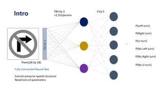
- 4. Intro Pixels(28 by 28) 784 by 3 =2,352params Fully Connected Neural Net 3 by 5 P(Left turn) P(Right turn) P(No Left turn) P(U-turn) P(No U-turn) P(No Right turn) … Cannot preserve spatial structure Need tons of parameters 784by1
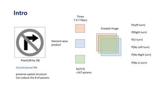
- 5. Intro Pixels(28 by 28) Convolutional NN P(Left turn) P(Right turn) P(No Left turn) P(U-turn) P(No U-turn) P(No Right turn) Three 7 X 7 filters preserve spatial structure Can reduce the # of params 3x(7x7) =147 params Created image Element-wise product
- 6. Intro Pixels(28 by 28) Use Filters! 7 by 7 filters
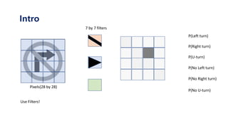
- 7. Intro Pixels(28 by 28) Use Filters! P(Left turn) P(Right turn) P(No Left turn) P(U-turn) P(No U-turn) P(No Right turn) 7 by 7 filters
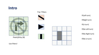
- 8. Intro Pixels(28 by 28) Use Filters! P(Left turn) P(Right turn) P(No Left turn) P(U-turn) P(No U-turn) P(No Right turn) 7 by 7 filters
- 9. Intro There is a diagonal line Right arrow signal on the upper right Vertical line on the mid-left Umm..
- 10. Intro There is a diagonal line Right arrow signal on the upper right Vertical line on the mid-left Must be ‘No turn right’ !
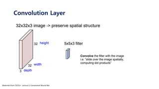
- 11. Convolution Layer Materials from CS231n : Lecture 5. Convolution Neural Net
- 12. Convolution Layer Materials from CS231n : Lecture 5. Convolution Neural Net
- 13. Convolution Layer Materials from CS231n : Lecture 5. Convolution Neural Net
- 14. Convolution Layer Materials from CS231n : Lecture 5. Convolution Neural Net
- 15. Convolution Layer Materials from CS231n : Lecture 5. Convolution Neural Net
- 16. Convolution Layer Materials from CS231n : Lecture 5. Convolution Neural Net
- 17. Convolution Layer 1 0 1 0 1 1 1 0 1 Filter http://deeplearning.stanford.edu/wiki/index.php/Feature_extraction_using_convolution https://cs.nyu.edu/~fergus/tutorials/deep_learning_cvpr12/
- 18. Convolution Layer Materials from CS231n : Lecture 5. Convolution Neural Net
- 19. Convolution Layer Materials from CS231n : Lecture 5. Convolution Neural Net
- 20. Convolution Layer In convolutional neural networks (CNN) every network layer acts as a detection filter for the presence of specific features or patterns present in the original data. The first layers(filters) in a CNN detect features that can be recognized and interpreted relatively easy. Later layers(filters) detect increasingly features that are more abstract.
- 21. Convolution Layer Test: Interpret first layers’ Filters Five 8X8 Filters FNCC Softmax Data Set: mnist 28x28x1
- 23. Convolution Layer Epoch: 200 Epoch: 600 Filters Initialize
- 24. Convolution Layer Filters Initialize Epoch: 200 Epoch: 600 Epoch: 5400 Epoch: 19800 Epoch: 1000 Epoch: 19800 Test accuracy: 0.9778
- 26. Convolution Layer paddingMax pool Size of next layer = (L-C+2P)/stride + 1
- 27. CNN Backprop Implementation - Computational Graphs - Backprop using for-loop - im2col
- 28. Computational Graphs A 𝜎 A soft max Loss func 𝑥 1 𝑊 1 𝑏 1 𝑊 2 𝑏 2 𝑥 2 𝑙𝑜𝑔𝑖𝑡𝑠 loss 𝑠𝑐𝑎𝑙𝑎𝑟 𝑙𝑎𝑏𝑒𝑙𝑠 𝑦𝑎 1 xW + 𝑏
- 29. Computational Graphs A 𝜎 A soft max Loss func 𝑥 1 𝑊 1 𝑏 1 𝑊 2 𝑏 2 𝑥 2 𝑙𝑜𝑔𝑖𝑡𝑠 1 𝑙𝑎𝑏𝑒𝑙𝑠 𝑦 𝜕𝐿/𝜕𝑦 loss 𝑠𝑐𝑎𝑙𝑎𝑟 𝑎 1
- 30. Computational Graphs A 𝜎 A soft max Loss func 𝑥 1 𝑊 1 𝑏 1 𝑊 2 𝑏 2 𝑥 2 𝑙𝑜𝑔𝑖𝑡𝑠 1 𝑙𝑎𝑏𝑒𝑙𝑠 𝑦 𝜕𝐿/𝜕𝑦 loss 𝑠𝑐𝑎𝑙𝑎𝑟 𝜕𝐿/𝜕𝑙𝑜𝑔𝑖𝑡𝑠 𝜕𝐿/𝜕𝑏 2 𝜕𝐿/𝜕𝑊 2 𝜕𝐿/𝜕𝑥 2 𝑎 1
- 31. Computational Graphs A 𝜎 A soft max Loss func 𝑥 1 𝑊 1 𝑏 1 𝑊 2 𝑏 2 𝑥 2 𝑙𝑜𝑔𝑖𝑡𝑠 1 𝑙𝑎𝑏𝑒𝑙𝑠 𝑦 𝜕𝐿/𝜕𝑦 loss 𝑠𝑐𝑎𝑙𝑎𝑟 𝜕𝐿/𝜕𝑙𝑜𝑔𝑖𝑡𝑠 𝜕𝐿/𝜕𝑏 2 𝜕𝐿/𝜕𝑊 2 𝜕𝐿/𝜕𝑥 2 𝑎 1 𝜕𝐿/𝜕𝑎 2 𝜕𝐿/𝜕𝑏 1 𝜕𝐿/𝜕𝑊 1
- 32. class Affine: def __init__(self,W,b): self.W = W self.b = b self.x = None self.dW = None self.db = None def forward(self,x): self.x = x out = np.dot(W,x) + self.b return out def backward(self,dout): self.db = np.sum(dout,axis=0) self.dW = np.dot(self.x.T,dout) dx = np.dot(dout,self.W.T) return dx A 𝑊 1 𝑏 1 Computational Graphs
- 33. class Affine: def __init__(self,W,b): self.W = W self.b = b self.x = None self.dW = None self.db = None def forward(self,x): self.x = x out = np.dot(W,x) + self.b return out def backward(self,dout): self.db = np.sum(dout,axis=0) self.dW = np.dot(self.x.T,dout) dx = np.dot(dout,self.W.T) return dx A 𝒙 𝟏 𝑊 1 𝑏 1 𝒂 𝟏 Computational Graphs 𝑖𝑛𝑝𝑢𝑡: 𝑜𝑢𝑡𝑝𝑢𝑡: xW + 𝑏
- 34. class Affine: def __init__(self,W,b): self.W = W self.b = b self.x = None self.dW = None self.db = None def forward(self,x): self.x = x out = np.dot(W,x) + self.b return out def backward(self,dout): self.db = np.sum(dout,axis=0) self.dW = np.dot(self.x.T,dout) dx = np.dot(dout,self.W.T) return dx A 𝑊 1 𝑏 1 Computational Graphs 𝑜𝑢𝑡𝑝𝑢𝑡: 𝑖𝑛𝑝𝑢𝑡: 𝝏𝑳/𝝏𝒂 𝝏𝑳/𝝏𝒙 𝝏𝑳/𝝏𝒃 𝝏𝑳/𝝏𝑾 𝒅𝒐𝒖𝒕 𝒙 𝟏
- 35. class Affine: def __init__(self,W,b): self.W = W self.b = b self.x = None self.dW = None self.db = None def forward(self,x): self.x = x out = np.dot(W,x) + self.b return out def backward(self,dout): self.db = np.sum(dout,axis=0) self.dW = np.dot(self.x.T,dout) dx = np.dot(dout,self.W.T) return dx A 𝑊 1 𝑏 1 Computational Graphs 𝑜𝑢𝑡𝑝𝑢𝑡: 𝑖𝑛𝑝𝑢𝑡: 𝝏𝑳/𝝏𝒂 𝝏𝑳/𝝏𝒙 𝝏𝑳/𝝏𝒃 𝝏𝑳/𝝏𝑾 𝒅𝒐𝒖𝒕 + + + 𝒙 𝟏 xW + 𝑏
- 36. class Affine: def __init__(self,W,b): self.W = W self.b = b self.x = None self.dW = None self.db = None def forward(self,x): self.x = x out = np.dot(W,x) + self.b return out def backward(self,dout): self.db = np.sum(dout,axis=0) self.dW = np.dot(self.x.T,dout) dx = np.dot(dout,self.W.T) return dx A 𝑊 1 𝑏 1 Computational Graphs 𝑖𝑛𝑝𝑢𝑡: 𝝏𝑳/𝝏𝒂 𝝏𝑳/𝝏𝒃 𝝏𝑳/𝝏𝑾 𝒅𝒐𝒖𝒕 𝐱 𝐭 × 𝒅𝒐𝒖𝒕 𝑜𝑢𝑡𝑝𝑢𝑡: 𝝏𝑳/𝝏𝒙 𝒙 𝟏 𝒅𝒐𝒖𝒕 × 𝐰 𝐭
- 37. Backprop Using for-Loop conv 𝜎 𝑥 1 𝑊 1 𝑥 2𝑎 1 Max pooling 𝑥 2 conv 𝑊 2 𝜎 𝑥 2 Max pooling
- 38. class Conv: def __init__(self,W): self.W = W self.x = None self.dW = None conv 𝑊 1 Backprop Using for-Loop
- 39. conv 𝑥 1 𝑊 1 𝑎 1 def forward(self,x): self.x = x #input과 filter의 column(=row) 크기 계산 size_x = self.x.shape[0] size_W = self.W.shape[0] #convolution 크기 계산후 생성 (x-w)/stride + 1 size_c = size_x - size_W + 1 conv_result = np.zeros(shape=(size_c,size_c)) #합성곱 연산 for i in range(size_c) : for j in range(size_c): partial = x[i:i+size_W , j:j+size_W] conv_result[i][j] = partial * size_W return conv_result Backprop Using for-Loop
- 40. conv 𝑥 1 𝑊 1 𝑎 1 def forward(self,x): self.x = x #input과 filter의 column(=row) 크기 계산 size_x = self.x.shape[0] size_W = self.W.shape[0] #convolution 크기 계산후 생성 (x-w)/stride + 1 size_c = size_x - size_W + 1 conv_result = np.zeros(shape=(size_c,size_c)) #합성곱 연산 for i in range(size_c) : for j in range(size_c): partial = x[i:i+size_W , j:j+size_W] conv_result[i][j] = partial * size_W return conv_result Backprop Using for-Loop
- 41. conv 𝑥 1 𝑊 1 𝑎 1 def forward(self,x): self.x = x #input과 filter의 column(=row) 크기 계산 size_x = self.x.shape[0] size_W = self.W.shape[0] #convolution 크기 계산후 생성 (x-w)/stride + 1 size_c = size_x - size_W + 1 conv_result = np.zeros(shape=(size_c,size_c)) #합성곱 연산 for i in range(size_c) : for j in range(size_c): partial = x[i:i+size_W , j:j+size_W] conv_result[i][j] = partial * size_W return conv_result Backprop Using for-Loop
- 42. X 𝑎 𝑐 Backprop Using for-Loop 𝑏 X 𝑎 𝑑𝐿 𝑑𝑐 𝑏 Before CNN Backprop..
- 43. X 𝑎 𝑐 Backprop Using for-Loop 𝑏 X 𝑎 𝑑𝐿 𝑑𝑐 𝑏 Before CNN Backprop.. 𝑑𝐿 𝑑𝑐 ∙ 𝑏 𝑑𝐿 𝑑𝑐 ∙ 𝑎
- 44. 𝑎(𝑚𝑎𝑡𝑟𝑖𝑥) 𝑐(scalar) Backprop Using for-Loop 𝑏(𝑚𝑎𝑡𝑟𝑖𝑥) conv 𝑎 𝑑𝐿 𝑑𝑐 𝑏 Before CNN Backprop.. conv 𝑎1 𝑏1 + 𝑎2 𝑏2 + 𝑎3 𝑏3 + ⋯ 𝑎 𝑛 𝑏 𝑛 = 𝑐
- 45. 𝑐(scalar) Backprop Using for-Loop conv 𝑎 𝑑𝐿 𝑑𝑐 𝑏 Before CNN Backprop.. 𝑑𝐿 𝑑𝑐 ∙ 𝑏 𝑑𝐿 𝑑𝑐 ∙ 𝑎 conv 𝑎(𝑚𝑎𝑡𝑟𝑖𝑥) 𝑏(𝑚𝑎𝑡𝑟𝑖𝑥) 𝑎1 𝑏1 + 𝑎2 𝑏2 + 𝑎3 𝑏3 + ⋯ 𝑎 𝑛 𝑏 𝑛 = 𝑐
- 46. conv 𝑥 1 𝑊 1 𝑎 1 def backward(self, dout): #input과 filter,x의 column(=row) 크기 계산 size_x = self.x.shape[0] #column(=row) 크기 size_W = self.W.shape[0] size_dout = dout.shape[0] #filter의 미분 결과 matrix self.dW = np.zeros(shape=(size_W,size_W)) #x의 미분 결과 matrix dx = np.zeros(shape=(size_x,size_x)) for i in range(size_dout) : for j in range(size_dout) : partial = self.x[i:i+size_W, j:j+size_W] self.dW += dout[i][j] * partial dx[i:i+size_W,j:j+size+W] += dout[i][j] * self.W return dx Backprop Using for-Loop
- 47. conv 𝑥 1 𝑊 1 𝑎 1 Backprop Using for-Loop def backward(self, dout): #input과 filter,x의 column(=row) 크기 계산 size_x = self.x.shape[0] #column(=row) 크기 size_W = self.W.shape[0] size_dout = dout.shape[0] #filter의 미분 결과 matrix self.dW = np.zeros(shape=(size_W,size_W)) #x의 미분 결과 matrix dx = np.zeros(shape=(size_x,size_x)) for i in range(size_dout) : for j in range(size_dout) : partial = self.x[i:i+size_W, j:j+size_W] self.dW += dout[i][j] * partial dx[i:i+size_W,j:j+size+W] += dout[i][j] * self.W return dx
- 48. conv 𝑥 1 𝑊 1 𝑎 1 Backprop Using for-Loop def backward(self, dout): #input과 filter,x의 column(=row) 크기 계산 size_x = self.x.shape[0] #column(=row) 크기 size_W = self.W.shape[0] size_dout = dout.shape[0] #filter의 미분 결과 matrix self.dW = np.zeros(shape=(size_W,size_W)) #x의 미분 결과 matrix dx = np.zeros(shape=(size_x,size_x)) for i in range(size_dout) : for j in range(size_dout) : partial = self.x[i:i+size_W, j:j+size_W] self.dW += dout[i][j] * partial dx[i:i+size_W,j:j+size+W] += dout[i][j] * self.W return dx
- 49. im2col There are highly optimized matrix multiplication routines for just about every platform(ex. Numpy) -> turn convolution into matrix multiplication!
- 50. im2col Materials from CS231n Winter : Lecture 11
- 51. im2col def im2col(input_data, filter_h, filter_w, stride=1, pad=0): """다수의 이미지를 입력받아 2차원 배열로 변환한다(평탄화). Parameters ---------- input_data : 4차원 배열 형태의 입력 데이터(이미지 수, 채널 수, 높이, 너비) filter_h : 필터의 높이 filter_w : 필터의 너비 stride : 스트라이드 pad : 패딩 Returns ------- col : 2차원 배열 """ N, C, H, W = input_data.shape out_h = (H + 2*pad - filter_h)//stride + 1 out_w = (W + 2*pad - filter_w)//stride + 1 img = np.pad(input_data, [(0,0), (0,0), (pad, pad), (pad, pad)], 'constant') col = np.zeros((N, C, filter_h, filter_w, out_h, out_w)) for y in range(filter_h): y_max = y + stride*out_h for x in range(filter_w): x_max = x + stride*out_w col[:, :, y, x, :, :] = img[:, :, y:y_max:stride, x:x_max:stride] col = col.transpose(0, 4, 5, 1, 2, 3).reshape(N*out_h*out_w, -1) return col https://github.com/WegraLee/deep-learning-from-scratch/blob/master/common/util.py
- 52. 10 Backprop Using for-Loop Simple 2 by 2 Max-pooling Max Pool 10 9 8 7 𝑦′Max Pool 𝑦′ 0 0 0
- 53. CNN in Practice Effective Receptive Field Bottleneck
- 54. input filter1 filter2 Effective Receptive Field
- 55. input Result 1 Receptive field : 3 by 3 Effective Receptive Field
- 56. input Result 1 Receptive field : 3 by 3 Result 2 Receptive field : 3 by 3 Effective Receptive Field
- 57. 1 9 input Result 1 1 2 3 4 5 6 7 8 9 Result 2 Effective Receptive field : 5 by 5 Effective Receptive Field
- 58. ERF : 5 X 5 ERF : 5 X 5 ERF : 5 X 5 ERF : 7 X 7 ERF : 7 X 7 Effective Receptive Field Materials from CS231n Winter : Lecture 11
- 59. ERF : 5 X 5 ERF : 5 X 5 ERF : 5 X 5 ERF : 7 X 7 ERF : 7 X 7 Effective Receptive Field Materials from CS231n Winter : Lecture 11
- 60. ERF : 5 X 5 ERF : 5 X 5 ERF : 5 X 5 ERF : 7 X 7 ERF : 7 X 7 Effective Receptive Field Materials from CS231n Winter : Lecture 11
- 61. ERF : 5 X 5 ERF : 5 X 5 ERF : 5 X 5 ERF : 7 X 7 ERF : 7 X 7 Fewer Parameters Less compute More nonlinearity GOOD! Effective Receptive Field Materials from CS231n Winter : Lecture 11
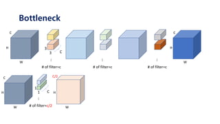
- 62. Bottleneck H W C
- 68. H W C … H W C # of filter=c 3 3 C … # of filter=c … # of filter=c Bottleneck
- 69. H W C … H W C # of filter=c 3 3 C … # of filter=c … # of filter=c H W C 1 1 C … # of filter=c/2 Bottleneck
- 70. H W C … H W C # of filter=c 3 3 C … # of filter=c … # of filter=c H W C 1 1 C … # of filter=c/2 C/2 H W Bottleneck
- 71. H W C … H W C # of filter=c 3 3 C … # of filter=c … # of filter=c H W C 1 1 C … # of filter=c/2 C/2 H W … # of filter=c/2 3 3 c/2 Bottleneck
- 72. H W C … H W C # of filter=c 3 3 C … # of filter=c … # of filter=c H W C 1 1 C … # of filter=c/2 C/2 H W … # of filter=c/2 3 3 c/2 Bottleneck
- 73. H W C … H W C # of filter=c 3 3 C … # of filter=c … # of filter=c H W C 1 1 C … # of filter=c/2 C/2 H W … # of filter=c/2 3 3 c/2 Bottleneck
- 74. H W C … H W C # of filter=c 3 3 C … # of filter=c … # of filter=c H W C 1 1 C … # of filter=c/2 C/2 H W … # of filter=c/2 3 3 c/2 1 1 C/2 … # of filter=c Bottleneck
- 75. H W C … H W C # of filter=c 3 3 C … # of filter=c … # of filter=c H W C 1 1 C … # of filter=c/2 C/2 H W … # of filter=c/2 3 3 c/2 1 1 C/2 … # of filter=c H W C Bottleneck
- 76. Materials from CS231n Winter : Lecture 11 Bottleneck
- 77. Materials from CS231n Winter : Lecture 11 Bottleneck
- 78. Materials from CS231n Winter : Lecture 11 Bottleneck
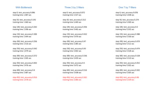
- 79. Bottleneck Test: Measure the duration(time) and accuracy of the model using bottleneck Data Set: CIFAR 10 32x32x3 , 10 labels 128 7x7x3 Filters Output: 32x32x128 Model 1 128 7x7x128 Filters Relu 1 layer Model 2 128 3x3x128 Filters Relu each time 3 layers Model 3 128 3x3x128 Filters 3 layers + bn & restore Total 5 layers Relu each time Input: 32x32x128 2by2 Max pooling Output: 16x16x128 FNCC & Softmax Epoch: 450 Batch size: 100 due to the environment condition
- 81. step 0, test_accuracy 0.078 training time 5.438 sec step 50, test_accuracy 0.274 training time 5.500 sec step 100, test_accuracy 0.4 training time 5.535 sec step 150, test_accuracy 0.388 training time 5.530 sec step 200, test_accuracy 0.474 training time 5.512 sec step 250, test_accuracy 0.474 training time 5.528 sec step 300, test_accuracy 0.528 training time 5.510 sec step 350, test_accuracy 0.452 training time 5.502 sec step 400, test_accuracy 0.502 training time 5.505 sec step 450, test_accuracy 0.48 training time 5.539 sec step 0, test_accuracy 0.072 training time 3.327 sec step 50, test_accuracy 0.312 training time 3.440 sec step 100, test_accuracy 0.356 training time 3.445 sec step 150, test_accuracy 0.432 training time 3.470 sec step 200, test_accuracy 0.47 training time 3.385 sec step 250, test_accuracy 0.43 training time 3.402 sec step 300, test_accuracy 0.536 training time 3.459 sec step 350, test_accuracy 0.5 training time 3.472 sec step 400, test_accuracy 0.516 training time 3.438 sec step 450, test_accuracy 0.562 training time 3.386 sec step 0, test_accuracy 0.096 training time 1.487 sec step 50, test_accuracy 0.192 training time 1.460 sec step 100, test_accuracy 0.262 training time 1.596 sec step 150, test_accuracy 0.306 training time 1.444 sec step 200, test_accuracy 0.356 training time 1.516 sec step 250, test_accuracy 0.342 training time 1.479 sec step 300, test_accuracy 0.372 training time 1.505 sec step 350, test_accuracy 0.402 training time 1.476 sec step 400, test_accuracy 0.4 training time 1.487 sec step 450, test_accuracy 0.416 training time 1.478 sec With Bottleneck Three 3 by 3 filters One 7 by 7 filters
- 82. Materials from CS231n Winter : Lecture 11 Bottleneck
- 83. CNN Architecture VGG/Inception/ResNet Materials from CS231n : Lecture 9. CNN Architecture
- 84. CNN Architecture Materials from CS231n : Lecture 9 CNN Architecture
- 85. VGG Materials from CS231n : Lecture 9 CNN Architecture
- 86. VGG Materials from CS231n : Lecture 9 CNN Architecture
- 87. Materials from CS231n : Lecture 9 CNN Architecture Inception
- 88. Materials from CS231n : Lecture 9 CNN Architecture Inception
- 89. Materials from CS231n : Lecture 9 CNN Architecture Inception
- 90. Materials from CS231n : Lecture 9 CNN Architecture Inception Auxiliary classification outputs to inject additional gradient at lower layers (AvgPool-1x1Conv-FC-FC-Softmax)
- 91. Materials from CS231n : Lecture 9 CNN Architecture ResNet
- 92. Materials from CS231n : Lecture 9 CNN Architecture ResNet
- 93. Materials from CS231n : Lecture 9 CNN Architecture ResNet
- 94. Materials from CS231n : Lecture 9 CNN Architecture ResNet
- 95. Most of Materials from CS231n References http://cs231n.stanford.edu/index.html Computational Graph 밑바닥부터 시작하는 딥러닝 https://github.com/WegraLee/deep-learning-from-scratch Inception Model https://norman3.github.io/papers/docs/google_inception.html Using tensorflow & tensorboard https://www.tensorflow.org/get_started/mnist/pros Tutorials & Programmer’s guide are really useful for me! https://ratsgo.github.io/deep%20learning/2017/04/05/CNNbackprop/