SlideShare a Scribd company logo
Uncertain Knowledge and Reasoning in Artificial Intelligence
Artificial Intelligence
Uncertain Knowledge and Reasoning
Andreas Haja
Prof. Dr. rer. nat.
Andreas Haja
Professor in Engineering
• My name is Dr. Andreas Haja and I am a
professor for engineering in Germany as
well as an expert for autonomous driving.
I worked for Volkswagen and Bosch as
project manager and research engineer.
• During my career, I developed algorithms to
track objects in videos, methods for vehicle
localization as well as prototype cars with
autonomous driving capabilities.
In many of these technical challenges,
artificial intelligence played a central role.
• In this course, I'd like to share with you my
10+ years of professional experience in the
field of AI gained in two of Germanys
largest engineering companies and in the
renowned elite University of Heidelberg.
Expert for Autonomous Cars
1. Welcome to this course!
2. Quantifying uncertainty
• Probability theory and Bayes’ rule
3. Representing uncertainty
• Bayesian networks and probability models
4. Final remarks
• Where to go from here?
Topics
Prerequisites
• This course is structured in a way that it is largely
complete in itself.
• For optimal benefit, a formal college education in
engineering, science or mathematics is
recommended.
• Helpful but not required is familiarity with computer
programming, preferably Python
• From stock investment to autonomous vehicles: Artificial intelligence takes the
world by storm. In many industries such as healthcare, transportation or finance,
smart algorithms have become an everyday reality. To be successful now and in
the future, companies need skilled professionals to understand and apply the
powerful tools offered by AI. This course will help you to achieve that goal.
• This practical guide offers a comprehensive overview of the most relevant AI
tools for reasoning under uncertainty. We will take a hands-on approach
interlaced with many examples, putting emphasis on easy understanding rather
than on mathematical formalities.
Course Description
• After this course, you will be able to...
• … understand different types of probabilities
• … use Bayes’ Rule as a problem-solving tool
• … leverage Python to directly apply the theories to practical problems
• … construct Bayesian networks to model complex decision problems
• … use Bayesian networks to perform inference and reasoning
• Wether you are an executive looking for a thorough overview of the subject, a
professional interested in refreshing your knowledge or a student planning on a
career into the field of AI, this course will help you to achieve your goals.
Course Description
• The opportunity to understand and explore one of the most
exciting advances in AI in the last decades
• A set of tools to model and process uncertain knowledge about
an environment and act on it
• A deep-dive into probabilities, Bayesian networks and inference
• Many hands-on examples, including Python code
• A firm foundation to further expand your knowledge in AI
What am I going to get from this course?
MODULE 1
Welcome to this course!
Introductory Example : Cancer or faulty test?
Module 1 10
• Imagine you are a doctor who has to conduct cancer screening to diagnose
patients. In one case, a patient is tested positive on cancer.
• You have the following background information:
o 1% of all people that are screened actually have cancer.
o 80% of all people who have cancer will test positive.
o 10% of people who do not have cancer will also test positive
• The patient is obviously very worried and wants to know the probability for him
actually having cancer, given the positive test result.
• Question : What is the probability for the test being correct?
Introductory Example : Cancer or faulty test?
Module 1 11
• What was your guess?
• Studies at Harvard Medical School have shown that 95 out of 100 physicians
estimated the probability for the patient actually having cancer to be between
70% and 80%.
• However, if you run the math, you arrive at only 8% instead. To be clear: In case
you are ever tested positive for cancer, your chances of not having it are above
90%.
• Probabilities are often counter-intuitive. Decisions based on uncertain
knowledge should thus be taken very carefully.
• Let’s take a look at how this can be done!
MODULE 2
Quantifying uncertainty
SECTION 1
Probability theory and Bayes’ rule
1. Intelligent agents
2. How to deal with uncertainty
o Example „Predicting a Burglary“
3. Basic probability theory
4. Conditional probabilities
5. Bayes’ rule
6. Example „Pedestrian detection sensor“
7. Example „Clinical trial“ (with Python code)
Probability theory and Bayes’ rule
Module 2 14
• At first some definitions:
o Intelligent agent : An autonomous entity in artificial intelligence
o Sensor : A device to detect events or changes in the environment
o Actor : A device which interacts with the environment
o Goal : A desired result that should be achieved in the future
• Intelligent agents observe the world through sensors and act on it using actuators.
Examples are e.g. autonomous vehicles or chat bots.
2. Quantifying Uncertainty - Intelligent Agents
https://www.doc.ic.ac.uk/project/examples/2005/163/g0516334/images/sensorseniv.pngModule 2 15
• The literature defines 5 types of agents which differ in their capabilities to arrive at
decisions based on internal structure and external stimuli.
• The simplest agent is the „simple reflex agent“ who functions according to a fixed set
of pre-defined condition-action rules.
2. Quantifying Uncertainty - Intelligent Agents
Module 2 15https://upload.wikimedia.org/wikipedia/commons/9/91/Simple_reflex_agent.png
• Simple reflex agents focus on current input. They can only succeed when the
environment is fully observable (which is rarely the case).
• A more sophisticated agent needs additional elements to deal with unknowns in its
environment:
o Model : A description of the world and how it works
o Goals : List of desirable states which the agent should achieve
o Utility : Maps information on agent „happiness“ (=utility) to each goal and allows a
comparison of different states according to their utility.
17
2. Quantifying Uncertainty - Intelligent Agents
Module 2
• A „model-based agent“ is able to function in environments which are only partially
observable. The agent maintains a model of how the world works and updates its
current state based on its observations.
18
https://upload.wikimedia.org/wikipedia/commons/8/8d/Model_based_reflex_agent.png
2. Quantifying Uncertainty - Intelligent Agents
Module 2
• In addition to a model of the world, a „goal-based agent“ maintains an idea of
desirable goals it tries to fulfil. This enables the agent to choose from several options,
choosing the one which reaches a goal state.
19
https://upload.wikimedia.org/wikipedia/commons/4/4f/Model_based_goal_based_agent.png
2. Quantifying Uncertainty - Intelligent Agents
Module 2
• A „utility-based agent“ bases its decisions on the expected utility of possible actions.
It needs information on utility of each outcome.
20
https://upload.wikimedia.org/wikipedia/commons/d/d8/Model_based_utility_based.png
2. Quantifying Uncertainty - Intelligent Agents
Module 2
• A „learning agent“ is able to operate in unknown environments and to improve its
actions over time. To learn, it uses feedback on how it is doing and modifies its
structure to increase future performance.
21
https://upload.wikimedia.org/wikipedia/commons/0/09/IntelligentAgent-Learning.png
2. Quantifying Uncertainty - Intelligent Agents
Module 2
• This lecture takes a close look at the inner workings of „utility-based agents“,
focussing at the problems of inference and reasoning.
22
https://upload.wikimedia.org/wikipedia/commons/d/d8/Model_based_utility_based.png
• Decision-making
• action selection
• Reasoning
• inference
2. Quantifying Uncertainty - Intelligent Agents
Module 2
1. In AI, an intelligent agent is an autonomous entity which observes the
world through sensors and acts upon it using actuators.
2. The literature lists five types of agents with the „simple reflex agent“
being the simplest and the „learning agent“ being the most complex.
3. This lecture focusses on the fundamentals behind the „utility-based
agent“ with a special emphasis on reasoning and inference.
Key Takeaways
2. Quantifying Uncertainty - Intelligent Agents
1. Intelligent agents
2. How to deal with uncertainty
o Example „Predicting a Burglary“
3. Basic probability theory
4. Conditional probabilities
5. Bayes’ rule
6. Example „Pedestrian detection sensor“
7. Example „Clinical trial“ (with Python code)
Probability theory and Bayes’ rule
Module 2 24
• Uncertainty […] describes a situation involving ambiguous and/or unknown
information. It applies to predictions of future events, to physical measurements that
are already made, or to the unknown.
[…]
It arises in any number of fields, including insurance, philosophy, physics, statistics,
economics, finance, psychology, sociology, engineering, metrology, meteorology,
ecology and information science.
• The proper handling of uncertainty is a prerequisite for artificial intelligence.
25
2. Quantifying Uncertainty - How to deal with uncertainty
[Wikipedia]
Module 2
• In reasoning and decision-making, uncertainty has many causes:
• Environment not fully observable
• Environment behaves in non-deterministic ways
• Actions might not have desired effects
• Reliance on default assumptions might not be justified
• Assumption: Agents which can reason about the effects of uncertainty should take
better decisions than agents who don’t.
• But : How should uncertainty be represented?
26
2. Quantifying Uncertainty - How to deal with uncertainty
Module 2
• Uncertainty can be addressed with two basic approaches:
o Extensional (logic-based)
o Intensional (probability-based)
27
2. Quantifying Uncertainty - How to deal with uncertainty
Module 2
• Before discussing a first example, let us define a number of basic terms required to
express uncertainty:
o Random variable : An observation or event with uncertain value
o Domain : Set of possible outcomes for a random variable
o Atomic event : State where all random variables have been resolved
28
2. Quantifying Uncertainty - How to deal with uncertainty
Module 2
• Before discussing a first example, let us define a number of basic terms required to
express uncertainty:
o Sentence : A logical combination of random variables
o Model : Set of atomic events that satisfies a specific sentence
o World : Set of all possible atomic events
o State of belief : Knowledge state based on received information
29
2. Quantifying Uncertainty - How to deal with uncertainty
Module 2
1. Intelligent agents
2. How to deal with uncertainty
o Example „Predicting a Burglary“
3. Basic probability theory
4. Conditional probabilities
5. Bayes’ rule
6. Example „Pedestrian detection sensor“
7. Example „Clinical trial“ (with Python code)
Probability theory and Bayes’ rule
Module 2 30
• Earthquake or burglary? (logic-based approach)
o Imagine you live in a house in San Francisco (or Tokyo) with a burglar alarm
installed. You know from experience that a minor earthquake may trigger the
alarm by mistake.
o Question : How can you know if there really was a burglary or not?
31
http://moziru.com/images/earthquake-clipart-symbol-png-9.png http://images.clipartpanda.com/burglary-clipart-6a00d83451586c69e2011570667cc6970b-320wi http://www.clker.com/cliparts/1/Z/i/2/V/v/orange-light-alarm-hi.png
2. Quantifying Uncertainty - Example „Predicting a Burglary“
Module 2
• What are the random variables and what are their domains?
• How many atomic events are there? 3 random variables —> 23 = 8
32
Atomic event Earthquake Burglary Alarm
a1 true true true
a2 true true false
a3 true false true
a4 true false false
a5 false true true
a6 false true false
a7 false false true
a8 false false false
2. Quantifying Uncertainty - Example „Predicting a Burglary“
Module 2
• Properties of the set of all atomic events (= the world):
o It is mutually exhaustive : No other permutations exist
o It is mutually exclusive : Only a single event can happen at a time
• How could a sentence look like?
o „Either an earthquake or a burglary entail an alarm.“
o „An Earthquake entails a Burglary.“
33
2. Quantifying Uncertainty - Example „Predicting a Burglary“
Module 2
• In propositional logic, there exist a number of logical connectives to combine two
variables P and Q:
• Let P be „Earthquake“ and Q be „Burglary“. Sentence s2 yields:
o 1 : If there is no earthquake then there is no burglary
o 2 : If there is no earthquake then there is a burglary
o 4 : If there is an earthquake, there is a burglary
34
Source: Artificial Intelligence - A modern approach (p. 246)
1
2
3
4
2. Quantifying Uncertainty - Example „Predicting a Burglary“
Module 2
• What would be models corresponding to the sentences?
o Applying the truth table to sentences s1 and s2 yields:
35
AE (E)arthqu. (B)urglary (A)larm E∨B E⇒B E∨B⇒A
a1 true true true true true true
a2 true true false true true false
a3 true false true true false true
a4 true false false true false false
a5 false true true true true true
a6 false true false true true false
a7 false false true false true true
a8 false false false false true true
2. Quantifying Uncertainty - Example „Predicting a Burglary“
Module 2
• Combining models corresponds to learning new information:
• The combined models provide the following atomic events:
o a1 : If there is an earthquake and a burglary, the alarm will sound.
o a5 : If there is no earthquake but a burglary, the alarm will sound.
o a7 : If there is no earthquake and no burglary, the alarm will sound.
o a8 : If there is no earthquake and no burglary, the alarm will not sound.
36
2. Quantifying Uncertainty - Example „Predicting a Burglary“
AE s2:
E⇒B
s1:
E∨B⇒A
a1 true true
a2 true false
a3 false true
a4 false false
a5 true true
a6 true false
a7 true true
a8 true true
Module 2
• Clearly, from the remaining atomic events, a7 does not make much sense. Also, it
is still impossible to trust the alarm as we do not know wether is has been
triggered by an earthquake or an actual burglary as stated by a1.
• Possible fix: Add more sentences to rule out unwanted atomic events.
• Problem:
o The world is complex and in most real-life scenarios, adding all the sentences
required for success is not feasible.
o There is no complete solution with logic (= qualification problem).
• Solution:
o Use probability theory to add sentences without explicitly naming them.
37
2. Quantifying Uncertainty - Example „Predicting a Burglary“
Module 2
1. Agents which can reason about the effects of uncertainty should take
better decisions than agents who don’t.
2. Uncertainty can be addressed with two basic approaches, logic-
based and probability-based.
3. Uncertainty is expressed with random variables. A set of random
variables with assigned values from their domains is an atomic event.
4. Random variables can be connected into sentences with logic. The
set of resulting atomic events is called a model.
5. Combining models corresponds to learning new information. In most
cases however, the world is too complex to be captured with logic.
Key Takeaways
2. Quantifying Uncertainty - Example „Predicting a Burglary“
1. Intelligent agents
2. How to deal with uncertainty
o Example „Predicting a Burglary“
3. Basic probability theory
4. Conditional probabilities
5. Bayes’ rule
6. Example „Pedestrian detection sensor“
7. Example „Clinical trial“ (with Python code)
Probability theory and Bayes’ rule
Module 2 39
• Probability can be expressed by expanding the domain of a random variable from a
discrete set {true, false} to a continuous set {0.0…1.0}.
• Probabilities can be seen as degrees of belief in atomic events:
40
AE Earthquake Burglary Alarm P(ai)
a1 true true true 0.0190
a2 true true false 0.0010
a3 true false true 0.0560
a4 true false false 0.0240
a5 false true true 0.1620
a6 false true false 0.0180
a7 false false true 0.0072
a8 false false false 0.7128
2. Quantifying Uncertainty - Basic probability theory
OR
AE E B A P(ai)
a1 1 1 1 0.0190
a2 1 1 0 0.0010
a3 1 0 1 0.0560
a4 1 0 0 0.0240
a5 0 1 1 0.1620
a6 0 1 0 0.0180
a7 0 0 1 0.0072
a8 0 0 0 0.7128
Module 2
• Expanding on P(a), probability can also be expressed as the degree of belief in a
specific sentence s and the models it entails:
• Example:
41
2. Quantifying Uncertainty - Basic probability theory
Module 2
• We can also express the probability of atomic events which share a specific state of
belief (e.g. earthquake = true):
• Note that the joint probability of all atomic events in world W must be 1:
42
2. Quantifying Uncertainty - Basic probability theory
AE E B A P(ai)
a1 1 1 1 0.0190
a2 1 1 0 0.0010
a3 1 0 1 0.0560
a4 1 0 0 0.0240
a5 0 1 1 0.1620
a6 0 1 0 0.0180
a7 0 0 1 0.0072
a8 0 0 0 0.7128
Module 2
• The concepts of probability theory can easily be visualized by using sets:
• Based on P(A) and P(B), the following junctions can be defined:
• Disjunction :
• Conjunction :
43
2. Quantifying Uncertainty - Basic probability theory
Module 2
• Based on random variables and atomic event probabilities, conjunction and
disjunction for earthquake and burglary are computed as:
44
2. Quantifying Uncertainty - Basic probability theory
AE E B A P(ai)
a1 1 1 1 0.0190
a2 1 1 0 0.0010
a3 1 0 1 0.0560
a4 1 0 0 0.0240
a5 0 1 1 0.1620
a6 0 1 0 0.0180
a7 0 0 1 0.0072
a8 0 0 0 0.7128
Module 2
1. Instead of expanding logic-based models with increasing complexity,
probabilities allow for shades of grey in between true and false.
2. Probabilities can be seen as degrees of belief in atomic events.
3. It is possible to compute the joint probability of a set of atomic events
which share a specific belief state by simply adding probabilities.
4. The joint probability of all atomic events must always add up to 1.
5. The probabilities of random variables can be combined using the
concepts of conjunctions and disjunctions.
Key Takeaways
2. Quantifying Uncertainty - Basic probability theory
1. Intelligent agents
2. How to deal with uncertainty
o Example „Predicting a Burglary“
3. Basic probability theory
4. Conditional probabilities
5. Bayes’ rule
6. Example „Pedestrian detection sensor“
7. Example „Clinical trial“ (with Python code)
Probability theory and Bayes’ rule
Module 2 46
• Based on the previously introduced truth table, we know the probabilities for Burglary
as well as for Burglary ∧ Alarm.
• Question: If we knew that there was an alarm, would that increase the probability of a
burglary? Intuitively, it would! But how to compute this?
47
2. Quantifying Uncertainty - Conditional probabilities
AE E B A P(ai)
a1 1 1 1 0.0190
a2 1 1 0 0.0010
a3 1 0 1 0.0560
a4 1 0 0 0.0240
a5 0 1 1 0.1620
a6 0 1 0 0.0180
a7 0 0 1 0.0072
a8 0 0 0 0.7128
Module 2
• If no further information exists about a random variable A, the associated probability is
called unconditional or prior probability P(A).
• In many cases, new information becomes available (through a random variable B) that
might change the probability of A (also: „the belief into A“).
• When such new information arrives, it is necessary to update the state of belief into A
by integrating B into the existing knowledge base.
• The resulting probability for the now dependent random variable A is called posterior
or conditional probability P(A | B) („probability for A given B“).
• Conditional probabilities reflect the fact that some events make others more or less
likely. Events that do not affect each other are independent.
48
2. Quantifying Uncertainty - Conditional probabilities
Module 2
• Conditional probabilities can be defined from unconditional probabilities:
• Expression (1) is also known as the product rule: For A and B to be both true, B must
be true and, given B, we also need A to be true.
• Alternative interpretation of (2) : A new belief state P(A|B) can be derived from the
joint probability of A and B, normalized with belief in new evidence.
• A belief update based on new evidence is called Bayesian conditioning.
49
2. Quantifying Uncertainty - Conditional probabilities
Module 2
• Example of Bayesian conditioning:
(first evidence)
50
2. Quantifying Uncertainty - Conditional probabilities
Given the evidence that the alarm is
triggered, the probability for a burglary
causing the alarm is at 74.1%.
AE E B A P(ai)
a1 1 1 1 0.0190
a2 1 1 0 0.0010
a3 1 0 1 0.0560
a4 1 0 0 0.0240
a5 0 1 1 0.1620
a6 0 1 0 0.0180
a7 0 0 1 0.0072
a8 0 0 0 0.7128
Module 2
• Example of Bayesian conditioning:
(second evidence)
51
Given the evidence that the alarm is triggered
during an earthquake, the probability for a
burglary causing the alarm is at 25.3%.
2. Quantifying Uncertainty - Conditional probabilities
AE E B A P(ai)
a1 1 1 1 0.0190
a2 1 1 0 0.0010
a3 1 0 1 0.0560
a4 1 0 0 0.0240
a5 0 1 1 0.1620
a6 0 1 0 0.0180
a7 0 0 1 0.0072
a8 0 0 0 0.7128
Module 2
• Clearly, Burglary and Earthquake should not be conditionally dependent.
But how can independence between two random variables be expressed?
• If event A is independent of event B, then the following relation holds:
• In the case of independence between two variables, an event B happening tells us
nothing about the event A. Therefore, the probability for B does not factor into the
computation of the probability of A.
52
2. Quantifying Uncertainty - Conditional probabilities
Module 2
1. If no further information exists about a random variable A, the
associated probability is called prior probability P(A).
2. If A is dependent on a second random variable B, the associated
probability is called conditional probability P(A | B).
3. Conditional probabilities can be defined from unconditional
probabilities using Bayesian conditioning.
4. Conditional probabilities allow for the integration of new information
or knowledge into a system.
5. If two events A and B are independent of each other, the probability
for event A is identical to the conditional probability of A given B.
Key Takeaways
2. Quantifying Uncertainty - Conditional probabilities
1. Intelligent agents
2. How to deal with uncertainty
o Example „Predicting a Burglary“
3. Basic probability theory
4. Conditional probabilities
5. Bayes’ rule
6. Example „Pedestrian detection sensor“
7. Example „Clinical trial“ (with Python code)
Probability theory and Bayes’ rule
Module 2 54
• Bayesian conditioning allows us to adjust the likelihood of an event A, given the
occurrence of another event B.
• Bayesian conditioning can also be interpreted as:
„Given a cause B, we can estimate the likelihood for an effect A“.
• But what if we observe an effect A and would like to know its cause?
55
caus
e
What we observe
effec
t
What we want to know
caus
e
effec
t
Bayesian
conditioning
???
2. Quantifying Uncertainty - Bayes’ Rule
Module 2
• In the last example of the burglary scenario, we observed the alarm and wanted to
know wether it had been caused by a burglary.
• But what if we wanted to reverse the question, i.e. how likely is it that the Alarm is
really triggered during a real burglary?
56
2. Quantifying Uncertainty - Bayes’ Rule
Module 2
• Based on the product rule, a new relationship between event B and event A can be
established. The result is known as Bayes’ rule:
• The order of events A and B in the product rule can be interchanged:
• As the two left-hand sides of (1) and (2) are identical, equating yields:
• After dividing both sides by P(A), we get Bayes’ rule:
57
2. Quantifying Uncertainty - Bayes’ Rule
Module 2
• Bayes’ rule is often termed one of the cornerstones of modern AI.
• But why is it so useful?
• If we model how likely an observable effect (e.g. Alarm) is based on a hidden cause
(e.g. Burglary), Bayes’ rule allows us to infer the likelihood of the hidden cause and
thus:
58
2. Quantifying Uncertainty - Bayes’ Rule
Module 2
• In the burglary scenario, we can now use Bayes’ rule to compute the conditional
probability of Alarm given Burglary as
• Using the results from the previous section, we get
• We now know that there was a 90% chance that the alarm would sound in case of a
burglary.
59
2. Quantifying Uncertainty - Bayes’ Rule
Module 2
1. Using Bayes’ Rule, we can reverse the order between what we
observe and what we want to know.
2. Bayes’ Rule is one of the cornerstones of modern AI as it allows for
probabilistic inference in many scenarios, e.g. in medicine.
Key Takeaways
2. Quantifying Uncertainty - Bayes’ Rule
1. Intelligent agents
2. How to deal with uncertainty
o Example „Predicting a Burglary“
3. Basic probability theory
4. Conditional probabilities
5. Bayes’ rule
6. Example „Pedestrian detection sensor“
7. Example „Clinical trial“ (with Python code)
Probability theory and Bayes’ rule
Module 2 61
• Example:
o An autonomous vehicle is equipped with a sensor that is able to detect
pedestrians. Once a pedestrian is detected, the vehicle will brake. However, in
some cases, the sensor will not work correctly.
62
https://www.volpe.dot.gov/sites/volpe.dot.gov/files/pictures/pedestrians-crosswalk-18256202_DieterHawlan-ml-500px.jpg
2. Quantifying Uncertainty - Example „Pedestrian detection sensor“
Module 2
• The sensor output may be divided into 4 different cases:
o True Positive (TP) : Pedestrian present, sensor gives an alarm
o True Negative (TN) : No pedestrian, sensor detects nothing
o False Positive (FP) : No pedestrian, sensor gives an alarm
o False Negative (FN) : Pedestrian present, sensor detects nothing
• Scenario : The sensor gives an alarm. Its false positive rate is 0.1% and the false
negative rate is 0.2%. On average, a pedestrian steps in front of a vehicle once in
every 1000km of driving.
• Question: How strong is our belief in the sensor alarm?
63
OK
ERROR
2. Quantifying Uncertainty - Example „Pedestrian detection sensor“
Module 2
• Based on the scenario description we may deduce:
o The probability for a pedestrian stepping in front of a car is :
o The probability for (inadvertently) braking, given there is no pedestrian is:
o Based on the false positive rate, it follows that in 99.1% of all cases where there is
no pedestrian in front of the car, the car will not brake:
64
2. Quantifying Uncertainty - Example „Pedestrian detection sensor“
Module 2
• Furthermore, it follows from the scenario description :
o The probability for not braking, even though there is a pedestrian, is :
o Based on the false negative rate, it follows that in 99.8% of all cases where there
is a pedestrian in front of the car, the car will brake:
o In all of the above cases, the classification into true/false negative/positive is
based on the knowledge wether there is a pedestrian or not (=ground truth).
65
2. Quantifying Uncertainty - Example „Pedestrian detection sensor“
Module 2
• In practice, knowledge wether there is a pedestrian is unavailable. The car has to rely
solely on its sensors to decide wether to brake or not.
• To assess the effectiveness of the sensor, it would be helpful to know the probability
of a correct braking decision, given there is a pedestrian.
• Using Bayes’ rule we can reverse the order of cause (pedestrian) and effect (braking
decision) to answer this question:
66
2. Quantifying Uncertainty - Example „Pedestrian detection sensor“
Module 2
• However, the probability for the vehicle braking is unknown. Given the true positive
rate as well as the false positive rate though, it can be computed as:
• Thus, during 1km of driving, the probability for the vehicle braking for a pedestrian
either correctly or inadvertently is 0.1997%.
67
2. Quantifying Uncertainty - Example „Pedestrian detection sensor“
Module 2
• The probability for a pedestrian actually being there when the car has decided to
issue a brake can now be computed using Bayes’ rule:
• If a pedestrian were to appear with P(pedestrian)=1/10.000 instead, the rarity of this
event would cause the probability to drop significantly:
68
2. Quantifying Uncertainty - Example „Pedestrian detection sensor“
Module 2
1. Intelligent agents
2. How to deal with uncertainty
o Example „Predicting a Burglary“
3. Basic probability theory
4. Conditional probabilities
5. Bayes’ rule
6. Example „Pedestrian detection sensor“
7. Example „Clinical trial“ (with Python code)
Probability theory and Bayes’ rule
Module 2 69
• Example:
o In a clinical trial, a student is first blindfolded and then asked to pick a pill at
random from one of two jars. Jar 1 is filled with 30 pills containing an active
substance and 10 placebos. Jar 2 contains 30 pills and 20 placebos.
o Afterwards, the student is told that he has picked a pill with an active
substance.
• Question: What is the probability that the pill has been picked from jar 1?
70
http://www.cityam.com/assets/uploads/main-image/cam_narrow_article_main_image/health-medecine-pills-151952018-56dda08258c8e.jpg
2. Quantifying Uncertainty - Example „Clinical trial“
Module 2
Probabilities from Bayes’ rule revisited:
• P(A) : Probability of choosing from a particular jar without any prior
evidence on what is selected (“prior probability”).
• P(B|A) : Conditional probability of selecting a pill or placebo given that we chose
to pick from a particular jar. Variable A holds the evidence.
• P(B) : Combined probabilities of selecting a pill or placebo from jar 1 or jar 2.
• P(A|B) : Probability of taking from a specific jar given that we picked a pill and not a
placebo or vice versa (“posterior probability“).
71
2. Quantifying Uncertainty - Example „Clinical trial“
Module 2
• Without any further information, we have to assume that the probability of selecting
from either jar1 or jar2 is equal :
• If we pick from jar1, the conditional probability for selecting a pill is 30/40 :
• If we pick from jar2, the conditional probability of selecting a pill is 20/40 :
72
2. Quantifying Uncertainty - Example „Clinical trial“
Module 2
• In probability theory, the law of total probability expresses the probability of a specific
outcome which can be realized via several distinct events:
• The probability of selecting a pill from any jar is thus
• Using Bayes’ rule we get the probability that a pill is picked from jar1:
73
2. Quantifying Uncertainty - Example „Clinical trial“
Module 2
• To solve this problem in Python, we define a function that takes the contents of both
jars as well as the probabilities for picking from each jar:
• Next, we make sure that probabilities are normalized and parameters are treated as
floating point numbers:
74
def clinical_trial(jar1_content, jar2_content, jar_prob) :
"Compute probability for picking content from a specific jar."
"Assumes that jar_content is provided as [#pill,#placebos]."
jar1_content = [float(i) for i in jar1_content]
jar2_content = [float(i) for i in jar2_content]
2. Quantifying Uncertainty - Example „Clinical trial“
Module 2
• Next, we compute the probabilities for picking either from jar1 or from jar2, again
making sure that all numbers are treated as decimals:
• Based on the distribution of pills and placebos in each jar, we can compute the
conditional probabilities for picking a specific item given each jar:
75
p_a = [float(jar_prob[0]) / float(sum(jar_prob)), # p_jar1
float(jar_prob[1]) / float(sum(jar_prob))] # p_jar2
p_b_a = [jar1_content[0]/sum(jar1_content), # p_pill_jar1
jar2_content[0]/sum(jar2_content), # p_pill_jar2
jar1_content[1]/sum(jar1_content), # p_placebo_jar1
jar2_content[1]/sum(jar2_content)] # p_placebo_jar2
2. Quantifying Uncertainty - Example „Clinical trial“
Module 2
• By applying the law of total probability, we can compute the probability for picking
either a pill or a placebo from any jar:
• Lastly, we now are able to apply Bayes’ theorem to get the probabilities for having
picked from a specific jar, given we selected a pill or a placebo.
76
p_b = [p_b_a[0]*p_a[0] + p_b_a[1]*p_a[1], # p_pill
p_b_a[2]*p_a[0] + p_b_a[3]*p_a[1]] # p_placebo
p_b_a = [jar1_content[0]/sum(jar1_content), # p_pill_jar1
jar2_content[0]/sum(jar2_content), # p_pill_jar2
jar1_content[1]/sum(jar1_content), # p_placebo_jar1
jar2_content[1]/sum(jar2_content)] # p_placebo_jar2
2. Quantifying Uncertainty - Example „Clinical trial“
Module 2
• We now print our results using:
• The call clinical_trial([70,30], [50,50], [0.5,0.5]) finally produces:
77
res1 = "The probability of having picked from "
res2 = ["jar 1 given a pill is ",
"jar 2 given a pill is ",
"jar 1 given a placebo is ",
"jar 2 given a placebo is "]
for i in range(0, 4) :
print(res1+res2[i]+"{0:.3f}".format(p_a_b[i]))
The probability of having picked from jar 1 given a pill is 0.583
The probability of having picked from jar 2 given a pill is 0.417
The probability of having picked from jar 1 given a placebo is 0.375
The probability of having picked from jar 2 given a placebo is 0.625
2. Quantifying Uncertainty - Example „Clinical trial“
Module 2
MODULE 3
Representing uncertainty

More Related Content

What's hot (20)

PPTX
Knowledge representation
Md. Tanvir Masud
 
PPTX
DBSCAN : A Clustering Algorithm
Pınar Yahşi
 
PPTX
Dempster shafer theory
Dr. C.V. Suresh Babu
 
PDF
Informed search
Amit Kumar Rathi
 
PPTX
K means clustering
keshav goyal
 
PPTX
lazy learners and other classication methods
rajshreemuthiah
 
PPT
Hill climbing
Mohammad Faizan
 
ODP
NAIVE BAYES CLASSIFIER
Knoldus Inc.
 
PPTX
Local search algorithm
Megha Sharma
 
PDF
Artificial Intelligence Chap.5 : Uncertainty
Khushali Kathiriya
 
PPTX
Naïve Bayes Classifier Algorithm.pptx
Shubham Jaybhaye
 
PPTX
Knowledge representation in AI
Vishal Singh
 
PDF
Convolutional Neural Networks (CNN)
Gaurav Mittal
 
PDF
I. Mini-Max Algorithm in AI
vikas dhakane
 
PPT
Back propagation
Nagarajan
 
PPTX
Multilayer perceptron
omaraldabash
 
PDF
Artificial Intelligence - Hill climbing.
StephenTec
 
PPTX
Semantic net in AI
ShahDhruv21
 
PPTX
Bayesian Belief Network and its Applications.pptx
SamyakJain710491
 
PPTX
Fuzzy Logic ppt
Ritu Bafna
 
Knowledge representation
Md. Tanvir Masud
 
DBSCAN : A Clustering Algorithm
Pınar Yahşi
 
Dempster shafer theory
Dr. C.V. Suresh Babu
 
Informed search
Amit Kumar Rathi
 
K means clustering
keshav goyal
 
lazy learners and other classication methods
rajshreemuthiah
 
Hill climbing
Mohammad Faizan
 
NAIVE BAYES CLASSIFIER
Knoldus Inc.
 
Local search algorithm
Megha Sharma
 
Artificial Intelligence Chap.5 : Uncertainty
Khushali Kathiriya
 
Naïve Bayes Classifier Algorithm.pptx
Shubham Jaybhaye
 
Knowledge representation in AI
Vishal Singh
 
Convolutional Neural Networks (CNN)
Gaurav Mittal
 
I. Mini-Max Algorithm in AI
vikas dhakane
 
Back propagation
Nagarajan
 
Multilayer perceptron
omaraldabash
 
Artificial Intelligence - Hill climbing.
StephenTec
 
Semantic net in AI
ShahDhruv21
 
Bayesian Belief Network and its Applications.pptx
SamyakJain710491
 
Fuzzy Logic ppt
Ritu Bafna
 

Similar to Uncertain Knowledge and Reasoning in Artificial Intelligence (20)

PPTX
Lesson04-Uncertainty - Pt. 1 Probabilistic Methods.pptx
RicardoSanz19
 
PPTX
Uncertainty in computer agent - Copy.pptx
sarmadthaer991
 
PDF
Ways to Solve Problems with Uncertain Knowledge.pdf
mehakgulzar473
 
PDF
AI CHAPTER 7.pdf
VatsalAgola
 
PPTX
Uncertainty in AI
Amruth Veerabhadraiah
 
PDF
Principles of Health Informatics: Artificial intelligence and machine learning
Martin Chapman
 
PDF
Uncertainty
Tribhuvan University
 
PPTX
Artificial Intelligence and Machine Learning
ssuser1ecccc
 
PDF
Introduction to Artificial Intelligence
ananth
 
PDF
artificial intelligence 13-quantifying uncertainity.pdf
SupreethGowda24
 
PPT
Artificial Intelligence by B. Ravikumar
Garry D. Lasaga
 
PDF
Artificial Intelligence and The Complexity
Hendri Karisma
 
PPTX
How to implement artificial intelligence solutions
Carlos Toxtli
 
PDF
Artificial Intelligence: an introduction.pdf
Eleonora Ciceri
 
PDF
Lecture9 - Bayesian-Decision-Theory
Albert Orriols-Puig
 
PDF
Artificial intelligence professor jinsong dong 2 august 2017
Alanna Forde
 
PDF
Module - 4 Machine Learning -22ISE62.pdf
Dr. Shivashankar
 
PPTX
CS3491-Unit-2 Uncertainty.pptx
Srinivasan Lakshmanan
 
PDF
Modeling uncertainty in deep learning
Sungjoon Choi
 
PPTX
Artificial intelligence: Simulation of Intelligence
Abhishek Upadhyay
 
Lesson04-Uncertainty - Pt. 1 Probabilistic Methods.pptx
RicardoSanz19
 
Uncertainty in computer agent - Copy.pptx
sarmadthaer991
 
Ways to Solve Problems with Uncertain Knowledge.pdf
mehakgulzar473
 
AI CHAPTER 7.pdf
VatsalAgola
 
Uncertainty in AI
Amruth Veerabhadraiah
 
Principles of Health Informatics: Artificial intelligence and machine learning
Martin Chapman
 
Artificial Intelligence and Machine Learning
ssuser1ecccc
 
Introduction to Artificial Intelligence
ananth
 
artificial intelligence 13-quantifying uncertainity.pdf
SupreethGowda24
 
Artificial Intelligence by B. Ravikumar
Garry D. Lasaga
 
Artificial Intelligence and The Complexity
Hendri Karisma
 
How to implement artificial intelligence solutions
Carlos Toxtli
 
Artificial Intelligence: an introduction.pdf
Eleonora Ciceri
 
Lecture9 - Bayesian-Decision-Theory
Albert Orriols-Puig
 
Artificial intelligence professor jinsong dong 2 august 2017
Alanna Forde
 
Module - 4 Machine Learning -22ISE62.pdf
Dr. Shivashankar
 
CS3491-Unit-2 Uncertainty.pptx
Srinivasan Lakshmanan
 
Modeling uncertainty in deep learning
Sungjoon Choi
 
Artificial intelligence: Simulation of Intelligence
Abhishek Upadhyay
 
Ad

More from Experfy (20)

PPTX
Predictive Analytics and Modeling in Life Insurance
Experfy
 
PPTX
Predictive Analytics and Modeling in Product Pricing (Personal and Commercial...
Experfy
 
PPTX
Graph Models for Deep Learning
Experfy
 
PPTX
Apache HBase Crash Course - Quick Tutorial
Experfy
 
PPTX
Machine Learning in AI
Experfy
 
PPTX
A Gentle Introduction to Genomics
Experfy
 
PPTX
A Comprehensive Guide to Insurance Technology - InsurTech
Experfy
 
PPTX
Health Insurance 101
Experfy
 
PPTX
Financial Derivatives
Experfy
 
PPTX
AI for executives
Experfy
 
PPTX
Cloud Native Computing Foundation: How Virtualization and Containers are Chan...
Experfy
 
PPTX
Microsoft Azure Power BI
Experfy
 
PPTX
March Towards Big Data - Big Data Implementation, Migration, Ingestion, Manag...
Experfy
 
PPTX
Sales Forecasting
Experfy
 
PPTX
Unsupervised Learning: Clustering
Experfy
 
PPTX
Introduction to Healthcare Analytics
Experfy
 
PDF
Blockchain Technology Fundamentals
Experfy
 
PPTX
Data Quality: Are Your Data Suitable For Answering Your Questions? - Experfy ...
Experfy
 
PPTX
Apache Spark SQL- Installing Spark
Experfy
 
PDF
Econometric Analysis | Methods and Applications
Experfy
 
Predictive Analytics and Modeling in Life Insurance
Experfy
 
Predictive Analytics and Modeling in Product Pricing (Personal and Commercial...
Experfy
 
Graph Models for Deep Learning
Experfy
 
Apache HBase Crash Course - Quick Tutorial
Experfy
 
Machine Learning in AI
Experfy
 
A Gentle Introduction to Genomics
Experfy
 
A Comprehensive Guide to Insurance Technology - InsurTech
Experfy
 
Health Insurance 101
Experfy
 
Financial Derivatives
Experfy
 
AI for executives
Experfy
 
Cloud Native Computing Foundation: How Virtualization and Containers are Chan...
Experfy
 
Microsoft Azure Power BI
Experfy
 
March Towards Big Data - Big Data Implementation, Migration, Ingestion, Manag...
Experfy
 
Sales Forecasting
Experfy
 
Unsupervised Learning: Clustering
Experfy
 
Introduction to Healthcare Analytics
Experfy
 
Blockchain Technology Fundamentals
Experfy
 
Data Quality: Are Your Data Suitable For Answering Your Questions? - Experfy ...
Experfy
 
Apache Spark SQL- Installing Spark
Experfy
 
Econometric Analysis | Methods and Applications
Experfy
 
Ad

Recently uploaded (20)

PPTX
I AM MALALA The Girl Who Stood Up for Education and was Shot by the Taliban...
Beena E S
 
PPTX
How to Create a PDF Report in Odoo 18 - Odoo Slides
Celine George
 
PPTX
Neurodivergent Friendly Schools - Slides from training session
Pooky Knightsmith
 
PDF
community health nursing question paper 2.pdf
Prince kumar
 
PPTX
MENINGITIS: NURSING MANAGEMENT, BACTERIAL MENINGITIS, VIRAL MENINGITIS.pptx
PRADEEP ABOTHU
 
PDF
Women's Health: Essential Tips for Every Stage.pdf
Iftikhar Ahmed
 
PDF
The dynastic history of the Chahmana.pdf
PrachiSontakke5
 
PDF
Reconstruct, Restore, Reimagine: New Perspectives on Stoke Newington’s Histor...
History of Stoke Newington
 
PPTX
Growth and development and milestones, factors
BHUVANESHWARI BADIGER
 
PPTX
How to Set Up Tags in Odoo 18 - Odoo Slides
Celine George
 
PDF
The History of Phone Numbers in Stoke Newington by Billy Thomas
History of Stoke Newington
 
PDF
The-Ever-Evolving-World-of-Science (1).pdf/7TH CLASS CURIOSITY /1ST CHAPTER/B...
Sandeep Swamy
 
PDF
0725.WHITEPAPER-UNIQUEWAYSOFPROTOTYPINGANDUXNOW.pdf
Thomas GIRARD, MA, CDP
 
PPTX
Unit 2 COMMERCIAL BANKING, Corporate banking.pptx
AnubalaSuresh1
 
PDF
ARAL_Orientation_Day-2-Sessions_ARAL-Readung ARAL-Mathematics ARAL-Sciencev2.pdf
JoelVilloso1
 
PPTX
SPINA BIFIDA: NURSING MANAGEMENT .pptx
PRADEEP ABOTHU
 
PDF
CONCURSO DE POESIA “POETUFAS – PASSOS SUAVES PELO VERSO.pdf
Colégio Santa Teresinha
 
PPTX
CATEGORIES OF NURSING PERSONNEL: HOSPITAL & COLLEGE
PRADEEP ABOTHU
 
PDF
Isharyanti-2025-Cross Language Communication in Indonesian Language
Neny Isharyanti
 
PDF
Stokey: A Jewish Village by Rachel Kolsky
History of Stoke Newington
 
I AM MALALA The Girl Who Stood Up for Education and was Shot by the Taliban...
Beena E S
 
How to Create a PDF Report in Odoo 18 - Odoo Slides
Celine George
 
Neurodivergent Friendly Schools - Slides from training session
Pooky Knightsmith
 
community health nursing question paper 2.pdf
Prince kumar
 
MENINGITIS: NURSING MANAGEMENT, BACTERIAL MENINGITIS, VIRAL MENINGITIS.pptx
PRADEEP ABOTHU
 
Women's Health: Essential Tips for Every Stage.pdf
Iftikhar Ahmed
 
The dynastic history of the Chahmana.pdf
PrachiSontakke5
 
Reconstruct, Restore, Reimagine: New Perspectives on Stoke Newington’s Histor...
History of Stoke Newington
 
Growth and development and milestones, factors
BHUVANESHWARI BADIGER
 
How to Set Up Tags in Odoo 18 - Odoo Slides
Celine George
 
The History of Phone Numbers in Stoke Newington by Billy Thomas
History of Stoke Newington
 
The-Ever-Evolving-World-of-Science (1).pdf/7TH CLASS CURIOSITY /1ST CHAPTER/B...
Sandeep Swamy
 
0725.WHITEPAPER-UNIQUEWAYSOFPROTOTYPINGANDUXNOW.pdf
Thomas GIRARD, MA, CDP
 
Unit 2 COMMERCIAL BANKING, Corporate banking.pptx
AnubalaSuresh1
 
ARAL_Orientation_Day-2-Sessions_ARAL-Readung ARAL-Mathematics ARAL-Sciencev2.pdf
JoelVilloso1
 
SPINA BIFIDA: NURSING MANAGEMENT .pptx
PRADEEP ABOTHU
 
CONCURSO DE POESIA “POETUFAS – PASSOS SUAVES PELO VERSO.pdf
Colégio Santa Teresinha
 
CATEGORIES OF NURSING PERSONNEL: HOSPITAL & COLLEGE
PRADEEP ABOTHU
 
Isharyanti-2025-Cross Language Communication in Indonesian Language
Neny Isharyanti
 
Stokey: A Jewish Village by Rachel Kolsky
History of Stoke Newington
 

Uncertain Knowledge and Reasoning in Artificial Intelligence

  • 2. Artificial Intelligence Uncertain Knowledge and Reasoning Andreas Haja Prof. Dr. rer. nat.
  • 3. Andreas Haja Professor in Engineering • My name is Dr. Andreas Haja and I am a professor for engineering in Germany as well as an expert for autonomous driving. I worked for Volkswagen and Bosch as project manager and research engineer. • During my career, I developed algorithms to track objects in videos, methods for vehicle localization as well as prototype cars with autonomous driving capabilities. In many of these technical challenges, artificial intelligence played a central role. • In this course, I'd like to share with you my 10+ years of professional experience in the field of AI gained in two of Germanys largest engineering companies and in the renowned elite University of Heidelberg. Expert for Autonomous Cars
  • 4. 1. Welcome to this course! 2. Quantifying uncertainty • Probability theory and Bayes’ rule 3. Representing uncertainty • Bayesian networks and probability models 4. Final remarks • Where to go from here? Topics
  • 5. Prerequisites • This course is structured in a way that it is largely complete in itself. • For optimal benefit, a formal college education in engineering, science or mathematics is recommended. • Helpful but not required is familiarity with computer programming, preferably Python
  • 6. • From stock investment to autonomous vehicles: Artificial intelligence takes the world by storm. In many industries such as healthcare, transportation or finance, smart algorithms have become an everyday reality. To be successful now and in the future, companies need skilled professionals to understand and apply the powerful tools offered by AI. This course will help you to achieve that goal. • This practical guide offers a comprehensive overview of the most relevant AI tools for reasoning under uncertainty. We will take a hands-on approach interlaced with many examples, putting emphasis on easy understanding rather than on mathematical formalities. Course Description
  • 7. • After this course, you will be able to... • … understand different types of probabilities • … use Bayes’ Rule as a problem-solving tool • … leverage Python to directly apply the theories to practical problems • … construct Bayesian networks to model complex decision problems • … use Bayesian networks to perform inference and reasoning • Wether you are an executive looking for a thorough overview of the subject, a professional interested in refreshing your knowledge or a student planning on a career into the field of AI, this course will help you to achieve your goals. Course Description
  • 8. • The opportunity to understand and explore one of the most exciting advances in AI in the last decades • A set of tools to model and process uncertain knowledge about an environment and act on it • A deep-dive into probabilities, Bayesian networks and inference • Many hands-on examples, including Python code • A firm foundation to further expand your knowledge in AI What am I going to get from this course?
  • 9. MODULE 1 Welcome to this course!
  • 10. Introductory Example : Cancer or faulty test? Module 1 10 • Imagine you are a doctor who has to conduct cancer screening to diagnose patients. In one case, a patient is tested positive on cancer. • You have the following background information: o 1% of all people that are screened actually have cancer. o 80% of all people who have cancer will test positive. o 10% of people who do not have cancer will also test positive • The patient is obviously very worried and wants to know the probability for him actually having cancer, given the positive test result. • Question : What is the probability for the test being correct?
  • 11. Introductory Example : Cancer or faulty test? Module 1 11 • What was your guess? • Studies at Harvard Medical School have shown that 95 out of 100 physicians estimated the probability for the patient actually having cancer to be between 70% and 80%. • However, if you run the math, you arrive at only 8% instead. To be clear: In case you are ever tested positive for cancer, your chances of not having it are above 90%. • Probabilities are often counter-intuitive. Decisions based on uncertain knowledge should thus be taken very carefully. • Let’s take a look at how this can be done!
  • 13. SECTION 1 Probability theory and Bayes’ rule
  • 14. 1. Intelligent agents 2. How to deal with uncertainty o Example „Predicting a Burglary“ 3. Basic probability theory 4. Conditional probabilities 5. Bayes’ rule 6. Example „Pedestrian detection sensor“ 7. Example „Clinical trial“ (with Python code) Probability theory and Bayes’ rule Module 2 14
  • 15. • At first some definitions: o Intelligent agent : An autonomous entity in artificial intelligence o Sensor : A device to detect events or changes in the environment o Actor : A device which interacts with the environment o Goal : A desired result that should be achieved in the future • Intelligent agents observe the world through sensors and act on it using actuators. Examples are e.g. autonomous vehicles or chat bots. 2. Quantifying Uncertainty - Intelligent Agents https://www.doc.ic.ac.uk/project/examples/2005/163/g0516334/images/sensorseniv.pngModule 2 15
  • 16. • The literature defines 5 types of agents which differ in their capabilities to arrive at decisions based on internal structure and external stimuli. • The simplest agent is the „simple reflex agent“ who functions according to a fixed set of pre-defined condition-action rules. 2. Quantifying Uncertainty - Intelligent Agents Module 2 15https://upload.wikimedia.org/wikipedia/commons/9/91/Simple_reflex_agent.png
  • 17. • Simple reflex agents focus on current input. They can only succeed when the environment is fully observable (which is rarely the case). • A more sophisticated agent needs additional elements to deal with unknowns in its environment: o Model : A description of the world and how it works o Goals : List of desirable states which the agent should achieve o Utility : Maps information on agent „happiness“ (=utility) to each goal and allows a comparison of different states according to their utility. 17 2. Quantifying Uncertainty - Intelligent Agents Module 2
  • 18. • A „model-based agent“ is able to function in environments which are only partially observable. The agent maintains a model of how the world works and updates its current state based on its observations. 18 https://upload.wikimedia.org/wikipedia/commons/8/8d/Model_based_reflex_agent.png 2. Quantifying Uncertainty - Intelligent Agents Module 2
  • 19. • In addition to a model of the world, a „goal-based agent“ maintains an idea of desirable goals it tries to fulfil. This enables the agent to choose from several options, choosing the one which reaches a goal state. 19 https://upload.wikimedia.org/wikipedia/commons/4/4f/Model_based_goal_based_agent.png 2. Quantifying Uncertainty - Intelligent Agents Module 2
  • 20. • A „utility-based agent“ bases its decisions on the expected utility of possible actions. It needs information on utility of each outcome. 20 https://upload.wikimedia.org/wikipedia/commons/d/d8/Model_based_utility_based.png 2. Quantifying Uncertainty - Intelligent Agents Module 2
  • 21. • A „learning agent“ is able to operate in unknown environments and to improve its actions over time. To learn, it uses feedback on how it is doing and modifies its structure to increase future performance. 21 https://upload.wikimedia.org/wikipedia/commons/0/09/IntelligentAgent-Learning.png 2. Quantifying Uncertainty - Intelligent Agents Module 2
  • 22. • This lecture takes a close look at the inner workings of „utility-based agents“, focussing at the problems of inference and reasoning. 22 https://upload.wikimedia.org/wikipedia/commons/d/d8/Model_based_utility_based.png • Decision-making • action selection • Reasoning • inference 2. Quantifying Uncertainty - Intelligent Agents Module 2
  • 23. 1. In AI, an intelligent agent is an autonomous entity which observes the world through sensors and acts upon it using actuators. 2. The literature lists five types of agents with the „simple reflex agent“ being the simplest and the „learning agent“ being the most complex. 3. This lecture focusses on the fundamentals behind the „utility-based agent“ with a special emphasis on reasoning and inference. Key Takeaways 2. Quantifying Uncertainty - Intelligent Agents
  • 24. 1. Intelligent agents 2. How to deal with uncertainty o Example „Predicting a Burglary“ 3. Basic probability theory 4. Conditional probabilities 5. Bayes’ rule 6. Example „Pedestrian detection sensor“ 7. Example „Clinical trial“ (with Python code) Probability theory and Bayes’ rule Module 2 24
  • 25. • Uncertainty […] describes a situation involving ambiguous and/or unknown information. It applies to predictions of future events, to physical measurements that are already made, or to the unknown. […] It arises in any number of fields, including insurance, philosophy, physics, statistics, economics, finance, psychology, sociology, engineering, metrology, meteorology, ecology and information science. • The proper handling of uncertainty is a prerequisite for artificial intelligence. 25 2. Quantifying Uncertainty - How to deal with uncertainty [Wikipedia] Module 2
  • 26. • In reasoning and decision-making, uncertainty has many causes: • Environment not fully observable • Environment behaves in non-deterministic ways • Actions might not have desired effects • Reliance on default assumptions might not be justified • Assumption: Agents which can reason about the effects of uncertainty should take better decisions than agents who don’t. • But : How should uncertainty be represented? 26 2. Quantifying Uncertainty - How to deal with uncertainty Module 2
  • 27. • Uncertainty can be addressed with two basic approaches: o Extensional (logic-based) o Intensional (probability-based) 27 2. Quantifying Uncertainty - How to deal with uncertainty Module 2
  • 28. • Before discussing a first example, let us define a number of basic terms required to express uncertainty: o Random variable : An observation or event with uncertain value o Domain : Set of possible outcomes for a random variable o Atomic event : State where all random variables have been resolved 28 2. Quantifying Uncertainty - How to deal with uncertainty Module 2
  • 29. • Before discussing a first example, let us define a number of basic terms required to express uncertainty: o Sentence : A logical combination of random variables o Model : Set of atomic events that satisfies a specific sentence o World : Set of all possible atomic events o State of belief : Knowledge state based on received information 29 2. Quantifying Uncertainty - How to deal with uncertainty Module 2
  • 30. 1. Intelligent agents 2. How to deal with uncertainty o Example „Predicting a Burglary“ 3. Basic probability theory 4. Conditional probabilities 5. Bayes’ rule 6. Example „Pedestrian detection sensor“ 7. Example „Clinical trial“ (with Python code) Probability theory and Bayes’ rule Module 2 30
  • 31. • Earthquake or burglary? (logic-based approach) o Imagine you live in a house in San Francisco (or Tokyo) with a burglar alarm installed. You know from experience that a minor earthquake may trigger the alarm by mistake. o Question : How can you know if there really was a burglary or not? 31 http://moziru.com/images/earthquake-clipart-symbol-png-9.png http://images.clipartpanda.com/burglary-clipart-6a00d83451586c69e2011570667cc6970b-320wi http://www.clker.com/cliparts/1/Z/i/2/V/v/orange-light-alarm-hi.png 2. Quantifying Uncertainty - Example „Predicting a Burglary“ Module 2
  • 32. • What are the random variables and what are their domains? • How many atomic events are there? 3 random variables —> 23 = 8 32 Atomic event Earthquake Burglary Alarm a1 true true true a2 true true false a3 true false true a4 true false false a5 false true true a6 false true false a7 false false true a8 false false false 2. Quantifying Uncertainty - Example „Predicting a Burglary“ Module 2
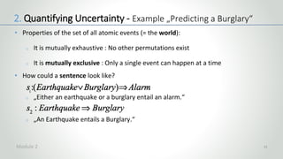
  • 33. • Properties of the set of all atomic events (= the world): o It is mutually exhaustive : No other permutations exist o It is mutually exclusive : Only a single event can happen at a time • How could a sentence look like? o „Either an earthquake or a burglary entail an alarm.“ o „An Earthquake entails a Burglary.“ 33 2. Quantifying Uncertainty - Example „Predicting a Burglary“ Module 2
  • 34. • In propositional logic, there exist a number of logical connectives to combine two variables P and Q: • Let P be „Earthquake“ and Q be „Burglary“. Sentence s2 yields: o 1 : If there is no earthquake then there is no burglary o 2 : If there is no earthquake then there is a burglary o 4 : If there is an earthquake, there is a burglary 34 Source: Artificial Intelligence - A modern approach (p. 246) 1 2 3 4 2. Quantifying Uncertainty - Example „Predicting a Burglary“ Module 2
  • 35. • What would be models corresponding to the sentences? o Applying the truth table to sentences s1 and s2 yields: 35 AE (E)arthqu. (B)urglary (A)larm E∨B E⇒B E∨B⇒A a1 true true true true true true a2 true true false true true false a3 true false true true false true a4 true false false true false false a5 false true true true true true a6 false true false true true false a7 false false true false true true a8 false false false false true true 2. Quantifying Uncertainty - Example „Predicting a Burglary“ Module 2
  • 36. • Combining models corresponds to learning new information: • The combined models provide the following atomic events: o a1 : If there is an earthquake and a burglary, the alarm will sound. o a5 : If there is no earthquake but a burglary, the alarm will sound. o a7 : If there is no earthquake and no burglary, the alarm will sound. o a8 : If there is no earthquake and no burglary, the alarm will not sound. 36 2. Quantifying Uncertainty - Example „Predicting a Burglary“ AE s2: E⇒B s1: E∨B⇒A a1 true true a2 true false a3 false true a4 false false a5 true true a6 true false a7 true true a8 true true Module 2
  • 37. • Clearly, from the remaining atomic events, a7 does not make much sense. Also, it is still impossible to trust the alarm as we do not know wether is has been triggered by an earthquake or an actual burglary as stated by a1. • Possible fix: Add more sentences to rule out unwanted atomic events. • Problem: o The world is complex and in most real-life scenarios, adding all the sentences required for success is not feasible. o There is no complete solution with logic (= qualification problem). • Solution: o Use probability theory to add sentences without explicitly naming them. 37 2. Quantifying Uncertainty - Example „Predicting a Burglary“ Module 2
  • 38. 1. Agents which can reason about the effects of uncertainty should take better decisions than agents who don’t. 2. Uncertainty can be addressed with two basic approaches, logic- based and probability-based. 3. Uncertainty is expressed with random variables. A set of random variables with assigned values from their domains is an atomic event. 4. Random variables can be connected into sentences with logic. The set of resulting atomic events is called a model. 5. Combining models corresponds to learning new information. In most cases however, the world is too complex to be captured with logic. Key Takeaways 2. Quantifying Uncertainty - Example „Predicting a Burglary“
  • 39. 1. Intelligent agents 2. How to deal with uncertainty o Example „Predicting a Burglary“ 3. Basic probability theory 4. Conditional probabilities 5. Bayes’ rule 6. Example „Pedestrian detection sensor“ 7. Example „Clinical trial“ (with Python code) Probability theory and Bayes’ rule Module 2 39
  • 40. • Probability can be expressed by expanding the domain of a random variable from a discrete set {true, false} to a continuous set {0.0…1.0}. • Probabilities can be seen as degrees of belief in atomic events: 40 AE Earthquake Burglary Alarm P(ai) a1 true true true 0.0190 a2 true true false 0.0010 a3 true false true 0.0560 a4 true false false 0.0240 a5 false true true 0.1620 a6 false true false 0.0180 a7 false false true 0.0072 a8 false false false 0.7128 2. Quantifying Uncertainty - Basic probability theory OR AE E B A P(ai) a1 1 1 1 0.0190 a2 1 1 0 0.0010 a3 1 0 1 0.0560 a4 1 0 0 0.0240 a5 0 1 1 0.1620 a6 0 1 0 0.0180 a7 0 0 1 0.0072 a8 0 0 0 0.7128 Module 2
  • 41. • Expanding on P(a), probability can also be expressed as the degree of belief in a specific sentence s and the models it entails: • Example: 41 2. Quantifying Uncertainty - Basic probability theory Module 2
  • 42. • We can also express the probability of atomic events which share a specific state of belief (e.g. earthquake = true): • Note that the joint probability of all atomic events in world W must be 1: 42 2. Quantifying Uncertainty - Basic probability theory AE E B A P(ai) a1 1 1 1 0.0190 a2 1 1 0 0.0010 a3 1 0 1 0.0560 a4 1 0 0 0.0240 a5 0 1 1 0.1620 a6 0 1 0 0.0180 a7 0 0 1 0.0072 a8 0 0 0 0.7128 Module 2
  • 43. • The concepts of probability theory can easily be visualized by using sets: • Based on P(A) and P(B), the following junctions can be defined: • Disjunction : • Conjunction : 43 2. Quantifying Uncertainty - Basic probability theory Module 2
  • 44. • Based on random variables and atomic event probabilities, conjunction and disjunction for earthquake and burglary are computed as: 44 2. Quantifying Uncertainty - Basic probability theory AE E B A P(ai) a1 1 1 1 0.0190 a2 1 1 0 0.0010 a3 1 0 1 0.0560 a4 1 0 0 0.0240 a5 0 1 1 0.1620 a6 0 1 0 0.0180 a7 0 0 1 0.0072 a8 0 0 0 0.7128 Module 2
  • 45. 1. Instead of expanding logic-based models with increasing complexity, probabilities allow for shades of grey in between true and false. 2. Probabilities can be seen as degrees of belief in atomic events. 3. It is possible to compute the joint probability of a set of atomic events which share a specific belief state by simply adding probabilities. 4. The joint probability of all atomic events must always add up to 1. 5. The probabilities of random variables can be combined using the concepts of conjunctions and disjunctions. Key Takeaways 2. Quantifying Uncertainty - Basic probability theory
  • 46. 1. Intelligent agents 2. How to deal with uncertainty o Example „Predicting a Burglary“ 3. Basic probability theory 4. Conditional probabilities 5. Bayes’ rule 6. Example „Pedestrian detection sensor“ 7. Example „Clinical trial“ (with Python code) Probability theory and Bayes’ rule Module 2 46
  • 47. • Based on the previously introduced truth table, we know the probabilities for Burglary as well as for Burglary ∧ Alarm. • Question: If we knew that there was an alarm, would that increase the probability of a burglary? Intuitively, it would! But how to compute this? 47 2. Quantifying Uncertainty - Conditional probabilities AE E B A P(ai) a1 1 1 1 0.0190 a2 1 1 0 0.0010 a3 1 0 1 0.0560 a4 1 0 0 0.0240 a5 0 1 1 0.1620 a6 0 1 0 0.0180 a7 0 0 1 0.0072 a8 0 0 0 0.7128 Module 2
  • 48. • If no further information exists about a random variable A, the associated probability is called unconditional or prior probability P(A). • In many cases, new information becomes available (through a random variable B) that might change the probability of A (also: „the belief into A“). • When such new information arrives, it is necessary to update the state of belief into A by integrating B into the existing knowledge base. • The resulting probability for the now dependent random variable A is called posterior or conditional probability P(A | B) („probability for A given B“). • Conditional probabilities reflect the fact that some events make others more or less likely. Events that do not affect each other are independent. 48 2. Quantifying Uncertainty - Conditional probabilities Module 2
  • 49. • Conditional probabilities can be defined from unconditional probabilities: • Expression (1) is also known as the product rule: For A and B to be both true, B must be true and, given B, we also need A to be true. • Alternative interpretation of (2) : A new belief state P(A|B) can be derived from the joint probability of A and B, normalized with belief in new evidence. • A belief update based on new evidence is called Bayesian conditioning. 49 2. Quantifying Uncertainty - Conditional probabilities Module 2
  • 50. • Example of Bayesian conditioning: (first evidence) 50 2. Quantifying Uncertainty - Conditional probabilities Given the evidence that the alarm is triggered, the probability for a burglary causing the alarm is at 74.1%. AE E B A P(ai) a1 1 1 1 0.0190 a2 1 1 0 0.0010 a3 1 0 1 0.0560 a4 1 0 0 0.0240 a5 0 1 1 0.1620 a6 0 1 0 0.0180 a7 0 0 1 0.0072 a8 0 0 0 0.7128 Module 2
  • 51. • Example of Bayesian conditioning: (second evidence) 51 Given the evidence that the alarm is triggered during an earthquake, the probability for a burglary causing the alarm is at 25.3%. 2. Quantifying Uncertainty - Conditional probabilities AE E B A P(ai) a1 1 1 1 0.0190 a2 1 1 0 0.0010 a3 1 0 1 0.0560 a4 1 0 0 0.0240 a5 0 1 1 0.1620 a6 0 1 0 0.0180 a7 0 0 1 0.0072 a8 0 0 0 0.7128 Module 2
  • 52. • Clearly, Burglary and Earthquake should not be conditionally dependent. But how can independence between two random variables be expressed? • If event A is independent of event B, then the following relation holds: • In the case of independence between two variables, an event B happening tells us nothing about the event A. Therefore, the probability for B does not factor into the computation of the probability of A. 52 2. Quantifying Uncertainty - Conditional probabilities Module 2
  • 53. 1. If no further information exists about a random variable A, the associated probability is called prior probability P(A). 2. If A is dependent on a second random variable B, the associated probability is called conditional probability P(A | B). 3. Conditional probabilities can be defined from unconditional probabilities using Bayesian conditioning. 4. Conditional probabilities allow for the integration of new information or knowledge into a system. 5. If two events A and B are independent of each other, the probability for event A is identical to the conditional probability of A given B. Key Takeaways 2. Quantifying Uncertainty - Conditional probabilities
  • 54. 1. Intelligent agents 2. How to deal with uncertainty o Example „Predicting a Burglary“ 3. Basic probability theory 4. Conditional probabilities 5. Bayes’ rule 6. Example „Pedestrian detection sensor“ 7. Example „Clinical trial“ (with Python code) Probability theory and Bayes’ rule Module 2 54
  • 55. • Bayesian conditioning allows us to adjust the likelihood of an event A, given the occurrence of another event B. • Bayesian conditioning can also be interpreted as: „Given a cause B, we can estimate the likelihood for an effect A“. • But what if we observe an effect A and would like to know its cause? 55 caus e What we observe effec t What we want to know caus e effec t Bayesian conditioning ??? 2. Quantifying Uncertainty - Bayes’ Rule Module 2
  • 56. • In the last example of the burglary scenario, we observed the alarm and wanted to know wether it had been caused by a burglary. • But what if we wanted to reverse the question, i.e. how likely is it that the Alarm is really triggered during a real burglary? 56 2. Quantifying Uncertainty - Bayes’ Rule Module 2
  • 57. • Based on the product rule, a new relationship between event B and event A can be established. The result is known as Bayes’ rule: • The order of events A and B in the product rule can be interchanged: • As the two left-hand sides of (1) and (2) are identical, equating yields: • After dividing both sides by P(A), we get Bayes’ rule: 57 2. Quantifying Uncertainty - Bayes’ Rule Module 2
  • 58. • Bayes’ rule is often termed one of the cornerstones of modern AI. • But why is it so useful? • If we model how likely an observable effect (e.g. Alarm) is based on a hidden cause (e.g. Burglary), Bayes’ rule allows us to infer the likelihood of the hidden cause and thus: 58 2. Quantifying Uncertainty - Bayes’ Rule Module 2
  • 59. • In the burglary scenario, we can now use Bayes’ rule to compute the conditional probability of Alarm given Burglary as • Using the results from the previous section, we get • We now know that there was a 90% chance that the alarm would sound in case of a burglary. 59 2. Quantifying Uncertainty - Bayes’ Rule Module 2
  • 60. 1. Using Bayes’ Rule, we can reverse the order between what we observe and what we want to know. 2. Bayes’ Rule is one of the cornerstones of modern AI as it allows for probabilistic inference in many scenarios, e.g. in medicine. Key Takeaways 2. Quantifying Uncertainty - Bayes’ Rule
  • 61. 1. Intelligent agents 2. How to deal with uncertainty o Example „Predicting a Burglary“ 3. Basic probability theory 4. Conditional probabilities 5. Bayes’ rule 6. Example „Pedestrian detection sensor“ 7. Example „Clinical trial“ (with Python code) Probability theory and Bayes’ rule Module 2 61
  • 62. • Example: o An autonomous vehicle is equipped with a sensor that is able to detect pedestrians. Once a pedestrian is detected, the vehicle will brake. However, in some cases, the sensor will not work correctly. 62 https://www.volpe.dot.gov/sites/volpe.dot.gov/files/pictures/pedestrians-crosswalk-18256202_DieterHawlan-ml-500px.jpg 2. Quantifying Uncertainty - Example „Pedestrian detection sensor“ Module 2
  • 63. • The sensor output may be divided into 4 different cases: o True Positive (TP) : Pedestrian present, sensor gives an alarm o True Negative (TN) : No pedestrian, sensor detects nothing o False Positive (FP) : No pedestrian, sensor gives an alarm o False Negative (FN) : Pedestrian present, sensor detects nothing • Scenario : The sensor gives an alarm. Its false positive rate is 0.1% and the false negative rate is 0.2%. On average, a pedestrian steps in front of a vehicle once in every 1000km of driving. • Question: How strong is our belief in the sensor alarm? 63 OK ERROR 2. Quantifying Uncertainty - Example „Pedestrian detection sensor“ Module 2
  • 64. • Based on the scenario description we may deduce: o The probability for a pedestrian stepping in front of a car is : o The probability for (inadvertently) braking, given there is no pedestrian is: o Based on the false positive rate, it follows that in 99.1% of all cases where there is no pedestrian in front of the car, the car will not brake: 64 2. Quantifying Uncertainty - Example „Pedestrian detection sensor“ Module 2
  • 65. • Furthermore, it follows from the scenario description : o The probability for not braking, even though there is a pedestrian, is : o Based on the false negative rate, it follows that in 99.8% of all cases where there is a pedestrian in front of the car, the car will brake: o In all of the above cases, the classification into true/false negative/positive is based on the knowledge wether there is a pedestrian or not (=ground truth). 65 2. Quantifying Uncertainty - Example „Pedestrian detection sensor“ Module 2
  • 66. • In practice, knowledge wether there is a pedestrian is unavailable. The car has to rely solely on its sensors to decide wether to brake or not. • To assess the effectiveness of the sensor, it would be helpful to know the probability of a correct braking decision, given there is a pedestrian. • Using Bayes’ rule we can reverse the order of cause (pedestrian) and effect (braking decision) to answer this question: 66 2. Quantifying Uncertainty - Example „Pedestrian detection sensor“ Module 2
  • 67. • However, the probability for the vehicle braking is unknown. Given the true positive rate as well as the false positive rate though, it can be computed as: • Thus, during 1km of driving, the probability for the vehicle braking for a pedestrian either correctly or inadvertently is 0.1997%. 67 2. Quantifying Uncertainty - Example „Pedestrian detection sensor“ Module 2
  • 68. • The probability for a pedestrian actually being there when the car has decided to issue a brake can now be computed using Bayes’ rule: • If a pedestrian were to appear with P(pedestrian)=1/10.000 instead, the rarity of this event would cause the probability to drop significantly: 68 2. Quantifying Uncertainty - Example „Pedestrian detection sensor“ Module 2
  • 69. 1. Intelligent agents 2. How to deal with uncertainty o Example „Predicting a Burglary“ 3. Basic probability theory 4. Conditional probabilities 5. Bayes’ rule 6. Example „Pedestrian detection sensor“ 7. Example „Clinical trial“ (with Python code) Probability theory and Bayes’ rule Module 2 69
  • 70. • Example: o In a clinical trial, a student is first blindfolded and then asked to pick a pill at random from one of two jars. Jar 1 is filled with 30 pills containing an active substance and 10 placebos. Jar 2 contains 30 pills and 20 placebos. o Afterwards, the student is told that he has picked a pill with an active substance. • Question: What is the probability that the pill has been picked from jar 1? 70 http://www.cityam.com/assets/uploads/main-image/cam_narrow_article_main_image/health-medecine-pills-151952018-56dda08258c8e.jpg 2. Quantifying Uncertainty - Example „Clinical trial“ Module 2
  • 71. Probabilities from Bayes’ rule revisited: • P(A) : Probability of choosing from a particular jar without any prior evidence on what is selected (“prior probability”). • P(B|A) : Conditional probability of selecting a pill or placebo given that we chose to pick from a particular jar. Variable A holds the evidence. • P(B) : Combined probabilities of selecting a pill or placebo from jar 1 or jar 2. • P(A|B) : Probability of taking from a specific jar given that we picked a pill and not a placebo or vice versa (“posterior probability“). 71 2. Quantifying Uncertainty - Example „Clinical trial“ Module 2
  • 72. • Without any further information, we have to assume that the probability of selecting from either jar1 or jar2 is equal : • If we pick from jar1, the conditional probability for selecting a pill is 30/40 : • If we pick from jar2, the conditional probability of selecting a pill is 20/40 : 72 2. Quantifying Uncertainty - Example „Clinical trial“ Module 2
  • 73. • In probability theory, the law of total probability expresses the probability of a specific outcome which can be realized via several distinct events: • The probability of selecting a pill from any jar is thus • Using Bayes’ rule we get the probability that a pill is picked from jar1: 73 2. Quantifying Uncertainty - Example „Clinical trial“ Module 2
  • 74. • To solve this problem in Python, we define a function that takes the contents of both jars as well as the probabilities for picking from each jar: • Next, we make sure that probabilities are normalized and parameters are treated as floating point numbers: 74 def clinical_trial(jar1_content, jar2_content, jar_prob) : "Compute probability for picking content from a specific jar." "Assumes that jar_content is provided as [#pill,#placebos]." jar1_content = [float(i) for i in jar1_content] jar2_content = [float(i) for i in jar2_content] 2. Quantifying Uncertainty - Example „Clinical trial“ Module 2
  • 75. • Next, we compute the probabilities for picking either from jar1 or from jar2, again making sure that all numbers are treated as decimals: • Based on the distribution of pills and placebos in each jar, we can compute the conditional probabilities for picking a specific item given each jar: 75 p_a = [float(jar_prob[0]) / float(sum(jar_prob)), # p_jar1 float(jar_prob[1]) / float(sum(jar_prob))] # p_jar2 p_b_a = [jar1_content[0]/sum(jar1_content), # p_pill_jar1 jar2_content[0]/sum(jar2_content), # p_pill_jar2 jar1_content[1]/sum(jar1_content), # p_placebo_jar1 jar2_content[1]/sum(jar2_content)] # p_placebo_jar2 2. Quantifying Uncertainty - Example „Clinical trial“ Module 2
  • 76. • By applying the law of total probability, we can compute the probability for picking either a pill or a placebo from any jar: • Lastly, we now are able to apply Bayes’ theorem to get the probabilities for having picked from a specific jar, given we selected a pill or a placebo. 76 p_b = [p_b_a[0]*p_a[0] + p_b_a[1]*p_a[1], # p_pill p_b_a[2]*p_a[0] + p_b_a[3]*p_a[1]] # p_placebo p_b_a = [jar1_content[0]/sum(jar1_content), # p_pill_jar1 jar2_content[0]/sum(jar2_content), # p_pill_jar2 jar1_content[1]/sum(jar1_content), # p_placebo_jar1 jar2_content[1]/sum(jar2_content)] # p_placebo_jar2 2. Quantifying Uncertainty - Example „Clinical trial“ Module 2
  • 77. • We now print our results using: • The call clinical_trial([70,30], [50,50], [0.5,0.5]) finally produces: 77 res1 = "The probability of having picked from " res2 = ["jar 1 given a pill is ", "jar 2 given a pill is ", "jar 1 given a placebo is ", "jar 2 given a placebo is "] for i in range(0, 4) : print(res1+res2[i]+"{0:.3f}".format(p_a_b[i])) The probability of having picked from jar 1 given a pill is 0.583 The probability of having picked from jar 2 given a pill is 0.417 The probability of having picked from jar 1 given a placebo is 0.375 The probability of having picked from jar 2 given a placebo is 0.625 2. Quantifying Uncertainty - Example „Clinical trial“ Module 2