SlideShare a Scribd company logo
THEORY OF
COMPUTATIO
N
Theory of Computation
• What?
• The theory of computation is a branch of computer science and
mathematics combined
• Deals with how efficiently problems can be solved on a model
of
computation, using an algorithm.
2
Application
• Where?
• Text processing
• Compilers
• Programming Languages
• Artificial Intelligence
• Genetic programming
• Neural Networks
• Robotics
3
Models
4
Models
5
UNIT I
AUTOMATA FUNDAMENTALS
Introduction to formal proof – Additional forms of Proof –
Inductive Proofs –Finite Automata – Deterministic Finite
Automata – Non-deterministic Finite Automata – Finite Automata
with Epsilon Transitions
6
Terminologies
• Alphabet
• Finite, non empty set of symbols
• Basic elements of a language
• Denoted by ∑
• String
• Finite sequence of symbols chosen from some alphabets
• Empty string
• Length of the string
• Power of an alphabet
• Language
• Set of all strings which are chosen from ∑*
7
Example
• English
• Alphabet – [a-z]
• String –{hi,hello,…}
• Binary number
• Alphabet – [0,1]
• String –{0,1,00,01,10,11…}
• Hexadecimal
• Alphabet –[0-9][a-e]
• String –[0,1,1A3,…]
8
Introduction to formal proof –
Additional forms of Proof –
Inductive Proofs
Introduction to Formal Proof
• Deductive Proof
• Reduction to definition
• Other theorem forms
• Theorem that appear not to be if-then statements
10
Deductive Proof
• A deductive proof consists of a sequence of statements whose
truth leads us from some initial statement called the
hypothesis or the given statement(s) to a conclusion
statement.
• Each step in the proof must follow by some accepted logical
principle from either the given facts or some of the previous
statement
• The hypothesis may be true or false, depending on the value
of its parameter
• If H then C . C is deducted from H
11
• Hypothesis : x ≥ 4
• Conclusion : 2x ≥
x2
• Parameter : x
• Proof:
• If x=3, then 23 ≥ 32 
• If x=4 then 24 ≥ 42 
8 ≥ 9 which is false
16 ≥ 16 which is true
• For each time x increments by 1, the LHS get incremented by 2
𝑥+
1�
�
2
and the RHS
• If x ≥ 4, the
𝑥+
1�
�
= 1.25, (1.25)2= 1.5625
• 1.5625 is less than 2
• Hence 2x ≥ x2 will be true for x ≥ 4 23
If x is the sum of the squares of four
positive integers, then 2x ≥ x2
13
Reduction to Definitions
• Convert all the terms in hypothesis to their definitions
• Deductive proof
14
Let S be a finite subset of some infinite
set U. Let T be the complement of S with
respect to U. Then T is infinite
• Let us assume T is finite, |T| = m
• As per the given statement, S is finite => |S|=n
• Then |S U T | = n+ m, which is finite which contradicts the
given statement, Hence T should be infinite. 26
Other Theorem Forms
• Ways of saying If-Then
• H implies C
• H only if C
• C if H
• Whenever H holds, C follows
• If and only if statement
• A if and only if B
• If part : If B then A
• Only if part: If A then B
16
Theorem that appear not to be
If- Then Statement
2
sin 𝛼 ± sin 𝛽 =
sin
𝛼
± 𝛽
co
s
• Example
𝑎2
+ 𝑏2
= 𝑐2
1 1
2
2
𝛼
∓ 𝛽
17
Additional Forms of Proof
• Proofs by sets
• Proof by Contrapositive
• Proofs by contradiction
• Proofs by counterexample
18
Proofs by sets
R U (S ∩ T) = (R U S) ∩ (R U T)
19
20
Proof by Contrapositive
• The contrapositive of a statement negates the conclusion as
well as the hypothesis. It is logically equivalent to the original
statement asserted. Often it is easier to prove the
contrapositive than the original statement.
• If H then C is equivalent to If not C then not H
• Example:
• If x ≥ 4 then 2x ≥ x2
• If not 2x ≥ x2 then not x ≥ 4
• If 2x < x2 then x < 4
21
Proofs by contradiction
• The method of proof by contradiction is to assume that a
statement is not true and then to show that that assumption
leads to a contradiction.
• To prove if H then C is to prove If H then not C
implies falsehood.
22
Proofs by counterexample
• A proof by counterexample is not technically a proof. It is
merely a way of showing that a given statement cannot
possibly be correct by showing an instance that contradicts a
universal statement.
• If integer x is a prime then x is odd
23
Inductive Proof
• Induction on integers
• Structural induction
• Mutual induction
24
Induction on integers
• Mathematical Induction is a mathematical technique which is
used to prove a statement, a formula or a theorem is true for
every natural number.
• The technique involves two steps to prove a statement, as
stated below −
• Step 1(Base step) − It proves that a statement is true for
the
initial value.
• Step 2(Inductive step) − It proves that if the statement is true
for the nth iteration (or number n), then it is also true for
(n+1)th iteration ( or number n+1).
25
1 + 2 + ... + n = n(n+1)/2
Proof. (Proof by Mathematical Induction)
Let's let P(n) be the statement "1 + 2 + ... + n = (n (n+1)/2."
Basis Step.
P(1) asserts "1 = 1(2)/2", which is clearly true. So we are done
with the initial step.
26
Inductive Step.
Induction Hypothesis/ Inductive assumption:
Assume, 1 + 2 + ... + k = k (k+1)/2 is true
Prove for k+1,
(i.e) 1 + 2 + ... + k + (k+1) = (k+1)(k+2)/2.
1 + 2 + ... + k + (k+1)
= k(k+1)/2 + (k+1)
= (k(k+1) + 2 (k+1))/2
= (k+1)(k+2)/2.
27
28
29
Structural Induction
• Structural induction is a proof methodology similar to
mathematical induction, only instead of working in the
domain of positive integers (N) it works in the domain of such
recursively defined structures!
• It is terrifically useful for proving properties of such
structures.
• Its structure is sometimes “looser” than that of mathematical
induction.
30
Every tree has one more node than its edges
• If T is a tree and T has n nodes and e edges then n=e+1
• Basis:
• T is single node tree, then n=1, e=0, so n=e+1 holds true
• Inductive Hypothesis:
• Assume the statement S(Ti ) hold for i=1,2,3,…,K and Ti have ni
nodes and ei edges then ni = ei + 1
• Induction
31
32
Every expression has an equal number of left and
right parentheses
• Let G is an expression
• Basis :
• G is a number or variable, so the number of left and right
parenthesis is 0
• Inductive Hypothesis:
• Assume E and F are two expressions which has equal
number of
left and right parentheses.
• Induction :
33
34
35
36
37
Finite Automata
• Finite automata are used to recognize patterns.
• It takes the string of symbol as input and changes its state
accordingly. When the desired symbol is found, then the
transition occurs.
• At the time of transition, the automata can either move to the
next state or stay in the same state.
• Finite automata have two states, Accept state or Reject state.
When the input string is processed successfully, and the
automata reached its final state, then it will accept.
38
• Input Tape
• It is a linear tape having some number of cells. Each input symbol is
placed in each cell.
• Finite control
• It decides the next state on receiving particular input from input
tape.
• Tape reader
• It reads the cells one by one from left to right, and at a time only
one input symbol is read.
39
• A finite automaton consists of:
• a finite set S of N states
• a special start state
• a set of final (or accepting) states
• a set of transitions T from one state to another, labelled with
chars in C
40
• Execution of FA on an input sequence as follows:
• Begin in the start state
• If the next input char matches the label on a transition from the
current state to a new state, go to that new state
• Continue making transitions on each input char
• If no move is possible, then stop
• If in accepting state, then accept
41
Deterministic Finite Automata
• Deterministic refers to the uniqueness of the computation.
• On each input there is one and only one state to which the
automaton can transition from its current state
• DFA does not accept the null move.
42
Formal Definition of DFA
• A deterministic finite automaton (DFA) is a 5-tuple
(Q,Σ,δ,q0,F),where
• Q is a finite set called the states,
• Σ is a finite set called the alphabet,
• δ:Q×Σ→Q is the transition function,
• q0 ∈ Q is the start state, and
• F ⊆ Q is the set of accepting states.
43
Transition Table
• A transition table is a tabular representation of the transition
function that takes two arguments and returns a state.
• The column contains the state in which the automaton will be
on the input represented by that column.
• The row corresponds to the state the finite control unit can
be
in.
• The entry for one row corresponding to state q and the
column corresponds to input a is the state δ(q, a).
44
Transition Diagram
• Transition graph can be interpreted as a flowchart for an
algorithm recognizing a language.
• A transition graph consists of three things:
• A finite set of states, at least one of which is designated the start
state and some of which are designated as final states.
• An alphabet Σ of possible input symbols from which the input
strings are formed.
• A finite set of transitions that show the change of state from the
given state on a given input.
45
Example DFA
states A b
q0 q1 q2
q1 q1 q3
q2 q2 q3
*q3 q3 q3
46
A=({q0,q1,q2,q3},{a,b}δ,q0,{q3})
δ is given by
δ(q0,a)=q1
δ(q0,b)=q2
δ(q1,a)=q1
δ(q2,b)=q2
δ(q1,b)=q3
δ(q2,a)=q3
δ(q3,a)=q3
δ(q3,b)=q3
• Design a DFA with ∑ = {0, 1} accepts those string which starts
with 1 and ends with 0.
• Design a DFA with ∑ = {0, 1} accepts the only input 101.
47
• Design a DFA with ∑ = {0, 1} accepts the strings with an even
number of 0's end by single 1.
48
Extended transition function
δ^
• The DFA define a language: the set of all strings that result in a
sequence of state transitions from the start state to an accepting
state
• Extended Transition Function
• Describes what happens when we start in any state and follow any
sequence of inputs
• If δ is our transition function, then the extended transition function is
denoted by δ^
• The extended transition function is a function that takes a state q and
a string w and returns a state p (the state that the automaton
reaches when starting in state q and processing the sequence of
inputs w)
• Let w=va then
60
δ(q, va) = δ(δ^ (q, v),
a).
Language accepted by DFA
• The language of a DFA A = (Q, Σ, δ, q0, F), denoted L(A) is
defined by
L(A) = { w | δ^(q0, w) is in F }
• The language of A is the set of strings w that take the start
state q0 to one of the accepting states
• If L is a L(A) from some DFA, then L is a regular language
50
Nondeterministic Finite
Automata
• An NFA is like a DFA, except that it can be in several states at
once.
• This can be seen as the ability to guess something about the
input.
• Useful for searching texts
51
Formal Definition of NFA
• A nondeterministic finite automaton (NFA) is a 5-tuple
(Q,Σ,δ,q0,F),where
• Q is a finite set called the states,
• Σ is a finite set called the alphabet,
• δ:Q×Σ→P(Q) is the transition function,
• q0 ∈ Q is the start state, and
• F ⊆ Q is the set of accepting states.
52
Extended transition function
δ^
• The extended transition function is a function that takes a
state q and a string w and returns a set of states P (The set of
possible state that the automaton reaches when starting in
state q and processing the sequence of inputs w)
• Let w=va then
δ^
𝑞0, 𝑣𝑎
= ∪ ′ ^
𝑞 ∈ δ
𝑞0,𝑣
δ( 𝑞
′,a)
53
Language accepted by NFA
• The language L(A) accepted by the NFA A is defined as follows:
L(A) = {w | δ^(q0, w) ∩ F ≠ ∅}
54
Example NFA
55
• Design an NFA with ∑ = {0, 1} in which double '1' is followed by
double '0'.
• Design an NFA with ∑ = {0, 1} accepts all string in which the
third symbol from the right end is always 0.
56
Epsilon Nondeterministic Finite
Automata
• Formal Definition
A ε-NFA is a quintuple A=(Q,Σ,δ,q0,F) where
• Q is a set of states
• Σ is the alphabet of input symbols
• ε is never a member of Σ. Σε is defined to be (Σ ∪ ε)
• δ: Q × Σε → P(Q) is the transition function
• q0 ∈ Q is the initial state
• F ⊆ Q is the set of final states
57
Example -
ε NFA
ε-NFA for a language which contain Os followed by 0 or more 1s.
58
-
ε closure
• Epsilon means present state can goto other state without any
input. This can happen only if the present state have epsilon
transition to other state.
• Epsilon closure is finding all the states which can be reached
from the present state on one or more epsilon transitions.
ε- closure (0)={0,1,2}
ε- closure(1)={1,2}
ε- closure(2)={2}
59
ε-closure of state a
60
ε-closure of state 0,1,2,3,4
61
62
δ^ - -
ε
NFA
𝑖=
1
δ^ 𝑞0,
𝑣𝑎 =
∪𝑘
𝑗=
1
δ(𝑝𝑖, 𝑎) =
∪𝑚
j
𝐸𝑐𝑙𝑜𝑠𝑒(
r )
Where δ (q0,v)= {p1,p2,…,pk }
& 𝑖=
1
∪𝑘 δ(𝑝𝑖, 𝑎)= {r1,r2,
…,rm }
63
Language accepted by -
ε NFA
The language of an ε-NFA E = (Q, Σ, δ, q0, F) is
L(E) = {w | ˆ δ(q0, w) ∩ F ≠ ∅}
64
Relationship between FAs
65
• Every DFA is NFA but not vice versa.
• Both NFA and DFA have same power and each NFA can be
translated into a DFA.
• There can be multiple final states in both DFA and NFA.
• NFA is more of a theoretical concept.
• DFA is used in Lexical Analysis in Compiler.
• Every NFA is ε-NFA but not vice-versa
66
Conversion of NFA to DFA
• Subset Construction Method
1. Create state table from the given NFA.
2. Create a blank state table under possible input alphabets for the
equivalent DFA.
3. Mark the start state of the DFA by q0 (Same as the NFA).
4. Find out the combination of States {Q0, Q1,... , Qn} for each
possible input alphabet.
5. Each time we generate a new DFA state under the input
alphabet columns, we have to apply step 4 again, otherwise go
to step 6.
6. The states which contain any of the final states of the NFA are
the final states of the equivalent DFA.
67
NFA
68
Subset construction
69
Transition Diagram for the
subset
70
Converted DFA
71
NFA  DFA
State 0 1
→q0 q0 q1
q1 {q1, q2} q1
*q2 q2 {q1, q2}
72
Now we will obtain δ' transition for state q0.
δ'([q0], 0) = [q0]
δ'([q0], 1) = [q1]
The δ' transition for state q1 is obtained as:
δ'([q1], 0) = [q1, q2] (new state generated)
δ'([q1], 1) = [q1]
73
Now we will obtain δ' transition on [q1, q2].
δ'([q1, q2], 0) = δ(q1, 0) ∪ δ(q2, 0)
= {q1, q2} ∪ {q2}
= [q1, q2]
δ'([q1, q2], 1) = δ(q1, 1) ∪ δ(q2,
1)
= {q1} ∪ {q1, q2}
= {q1, q2}
= [q1, q2]
The state [q1, q2] is the final state as well because
it contains a final state q2. 85
The transition table for the constructed DFA will
be:
State 0 1
→[q0] [q0] [q1]
[q1] [q1, q2] [q1]
*[q1, q2] [q1, q2] [q1, q2]
86
Conversion of -
ε NFA to DFA
• Modified subset construction
1. Find the ε-closure for the starting state of ε - NFA as a starting
state of DFA.
2. Find the states for each input symbol that can be traversed from
the present. That means the union of transition value and their
closures for each state of NFA present in the current state of
DFA.
3. If a new state is found, take it as current state and repeat step
2.
4. Repeat Step 2 and Step 3 until there is no new state present in
the transition table of DFA.
5. Mark the states of DFA as a final state which contains the final
state of ε-NFA. 87
Example
• Let us obtain ε-closure of each state.
ε-closure {q0} = {q0, q1, q2}
ε-closure {q1} = {q1}
ε-closure {q2} = {q2}
ε-closure {q3} = {q3}
ε-closure {q4} = {q4}
77
•let ε-closure {q0} = {q0, q1, q2} be state
A δ'(A, 0) = ε-closure {δ((q0, q1, q2), 0) }
= ε-closure {δ(q0, 0) ∪ δ(q1, 0) ∪
δ(q2, 0) }
= ε-closure {q3}
= {q3} call it as state B. δ'(A,
1) = ε-closure {δ((q0, q1, q2), 1) }
= ε-closure {δ((q0, 1)
∪ δ(q1, 1) ∪ δ(q2, 1)}
= ε-closure {q3}
= {q3} = B. 78
δ'(B, 0) = ε-closure {δ(q3, 0) }
= ϕ
δ'(B, 1) = ε-closure {δ(q3, 1) }
= ε-closure {q4}
= {q4}
i.e. state C
δ'(C, 0) = ε-closure {δ(q4, 0) }
= ϕ
δ'(C, 1) = ε-closure {δ(q4, 1) }
= ϕ
79
ε-closure(q0) = {q0, q1, q2}
ε-closure(q1) = {q1, q2}
ε-closure(q2) = {q2}
80
δ'(A, 0) = ε-closure{δ((q0, q1, q2), 0)}
= ε-closure{δ(q0, 0) ∪ δ(q1, 0) ∪ δ(q2,
0)}
= ε-closure{q0}
= {q0, q1, q2}
δ'(A, 1) = ε-closure{δ((q0, q1, q2), 1)}
= ε-closure{δ(q0, 1) ∪ δ(q1, 1) ∪ δ(q2,
1)}
= ε-closure{q1}
= {q1, q2} call it as state B
δ'(A, 2) = ε-closure{δ((q0, q1, q2), 2)}
= ε-closure{δ(q0, 2) ∪ δ(q1, 2) ∪ δ(q2,
2)}
= ε-closure{q2}
= {q2} call it state C
81
δ'(B, 0) = ε-closure{δ((q1, q2), 0)}
= ε-closure{δ(q1, 0) ∪ δ(q2,
0)}
= ε-closure{ϕ}
= ϕ
δ'(B, 1) = ε-closure{δ((q1, q2), 1)}
= ε-closure{δ(q1, 1) ∪ δ(q2,
1)}
= ε-closure{q1}
= {q1, q2} i.e.
state B itself
δ'(B, 2) = ε-closure{δ((q1, q2), 2)}
= ε-closure{δ(q1, 2) ∪ δ(q2,
2)}
= ε-closure{q2}
= {q2} i.e. state C
82
δ'(C, 0) = ε-closure{δ(q2, 0)}
= ε-closure{ϕ}
= ϕ
δ'(C, 1) = ε-closure{δ(q2, 1)}
= ε-closure{ϕ}
= ϕ
δ'(C, 2) = ε-closure{δ(q2, 2)}
= {q2}
83
ENFA to DFA
84

More Related Content

Similar to unit 1.pptx-theory of computation complete notes (20)

PPT
Introduction to the computing theory in automata
AbubakarSadiq69
 
PDF
Teori automata lengkap
Muhammad Love Kian
 
PPTX
IntroToAutomataTheory.pptx
PEzhumalai
 
PDF
Theory of Computation Lecture Notes
FellowBuddy.com
 
PPT
Intro automata theory
Rajendran
 
PPT
3.1 intro toautomatatheory h1
Rajendran
 
PPT
Dfa h11
Rajendran
 
PPTX
automata theory and formal languages Automata2Chapter1.pptx
ArjayBalberan1
 
PDF
Cs6503 theory of computation book notes
appasami
 
DOCX
Deterministic finite automata
Muhammad Love Kian
 
PDF
Unit i
TPLatchoumi
 
PPT
Flat
lavishka_anuj
 
PPTX
Unit -I Toc.pptx
viswanath kani
 
PPT
Finite automata intro
lavishka_anuj
 
PPT
Class1
issbp
 
PDF
Automata And Computability Solutions To Exercises Fall 2016
Jeff Nelson
 
PPT
rs1.ppt
ssuser47f7f2
 
PDF
Theory ofcomputation
nesrine attia
 
Introduction to the computing theory in automata
AbubakarSadiq69
 
Teori automata lengkap
Muhammad Love Kian
 
IntroToAutomataTheory.pptx
PEzhumalai
 
Theory of Computation Lecture Notes
FellowBuddy.com
 
Intro automata theory
Rajendran
 
3.1 intro toautomatatheory h1
Rajendran
 
Dfa h11
Rajendran
 
automata theory and formal languages Automata2Chapter1.pptx
ArjayBalberan1
 
Cs6503 theory of computation book notes
appasami
 
Deterministic finite automata
Muhammad Love Kian
 
Unit i
TPLatchoumi
 
Unit -I Toc.pptx
viswanath kani
 
Finite automata intro
lavishka_anuj
 
Class1
issbp
 
Automata And Computability Solutions To Exercises Fall 2016
Jeff Nelson
 
rs1.ppt
ssuser47f7f2
 
Theory ofcomputation
nesrine attia
 

More from yuvaraniit (8)

PPTX
unit 3.pptx-theory of computation unit 3 notes
yuvaraniit
 
PPTX
DSD Unit 1 Abstract Data Type data structures design notes.pptx
yuvaraniit
 
PPTX
fullunit2-220307090026 (1) theory of computation.pptx
yuvaraniit
 
PPTX
Class Orientation CS3452-Theory of computation.pptx
yuvaraniit
 
PPTX
OS UNIT-II-PPT.pptx-operating systems complete notes
yuvaraniit
 
PPTX
deadlock.pptx-operating systems -unit 2 notes
yuvaraniit
 
PPTX
1 UNIT I 3D graphics and game design.pptx
yuvaraniit
 
PPTX
UNIT 1 dbdm ad3391 unit lecture notes ppt
yuvaraniit
 
unit 3.pptx-theory of computation unit 3 notes
yuvaraniit
 
DSD Unit 1 Abstract Data Type data structures design notes.pptx
yuvaraniit
 
fullunit2-220307090026 (1) theory of computation.pptx
yuvaraniit
 
Class Orientation CS3452-Theory of computation.pptx
yuvaraniit
 
OS UNIT-II-PPT.pptx-operating systems complete notes
yuvaraniit
 
deadlock.pptx-operating systems -unit 2 notes
yuvaraniit
 
1 UNIT I 3D graphics and game design.pptx
yuvaraniit
 
UNIT 1 dbdm ad3391 unit lecture notes ppt
yuvaraniit
 
Ad

Recently uploaded (20)

PPTX
Lecture 1 Shell and Tube Heat exchanger-1.pptx
mailforillegalwork
 
PPTX
Heart Bleed Bug - A case study (Course: Cryptography and Network Security)
Adri Jovin
 
PDF
Design Thinking basics for Engineers.pdf
CMR University
 
PDF
GTU Civil Engineering All Semester Syllabus.pdf
Vimal Bhojani
 
PDF
Reasons for the succes of MENARD PRESSUREMETER.pdf
majdiamz
 
PDF
Viol_Alessandro_Presentazione_prelaurea.pdf
dsecqyvhbowrzxshhf
 
PPTX
Damage of stability of a ship and how its change .pptx
ehamadulhaque
 
PPT
Carmon_Remote Sensing GIS by Mahesh kumar
DhananjayM6
 
DOCX
CS-802 (A) BDH Lab manual IPS Academy Indore
thegodhimself05
 
PDF
MAD Unit - 1 Introduction of Android IT Department
JappanMavani
 
PPTX
Shinkawa Proposal to meet Vibration API670.pptx
AchmadBashori2
 
PPTX
Arduino Based Gas Leakage Detector Project
CircuitDigest
 
PPTX
Green Building & Energy Conservation ppt
Sagar Sarangi
 
PPTX
Introduction to Design of Machine Elements
PradeepKumarS27
 
PDF
Zilliz Cloud Demo for performance and scale
Zilliz
 
PPTX
DATA BASE MANAGEMENT AND RELATIONAL DATA
gomathisankariv2
 
PDF
Water Industry Process Automation & Control Monthly July 2025
Water Industry Process Automation & Control
 
PPTX
What is Shot Peening | Shot Peening is a Surface Treatment Process
Vibra Finish
 
PDF
Electrical Engineer operation Supervisor
ssaruntatapower143
 
PDF
Pressure Measurement training for engineers and Technicians
AIESOLUTIONS
 
Lecture 1 Shell and Tube Heat exchanger-1.pptx
mailforillegalwork
 
Heart Bleed Bug - A case study (Course: Cryptography and Network Security)
Adri Jovin
 
Design Thinking basics for Engineers.pdf
CMR University
 
GTU Civil Engineering All Semester Syllabus.pdf
Vimal Bhojani
 
Reasons for the succes of MENARD PRESSUREMETER.pdf
majdiamz
 
Viol_Alessandro_Presentazione_prelaurea.pdf
dsecqyvhbowrzxshhf
 
Damage of stability of a ship and how its change .pptx
ehamadulhaque
 
Carmon_Remote Sensing GIS by Mahesh kumar
DhananjayM6
 
CS-802 (A) BDH Lab manual IPS Academy Indore
thegodhimself05
 
MAD Unit - 1 Introduction of Android IT Department
JappanMavani
 
Shinkawa Proposal to meet Vibration API670.pptx
AchmadBashori2
 
Arduino Based Gas Leakage Detector Project
CircuitDigest
 
Green Building & Energy Conservation ppt
Sagar Sarangi
 
Introduction to Design of Machine Elements
PradeepKumarS27
 
Zilliz Cloud Demo for performance and scale
Zilliz
 
DATA BASE MANAGEMENT AND RELATIONAL DATA
gomathisankariv2
 
Water Industry Process Automation & Control Monthly July 2025
Water Industry Process Automation & Control
 
What is Shot Peening | Shot Peening is a Surface Treatment Process
Vibra Finish
 
Electrical Engineer operation Supervisor
ssaruntatapower143
 
Pressure Measurement training for engineers and Technicians
AIESOLUTIONS
 
Ad

unit 1.pptx-theory of computation complete notes

  • 2. Theory of Computation • What? • The theory of computation is a branch of computer science and mathematics combined • Deals with how efficiently problems can be solved on a model of computation, using an algorithm. 2
  • 3. Application • Where? • Text processing • Compilers • Programming Languages • Artificial Intelligence • Genetic programming • Neural Networks • Robotics 3
  • 6. UNIT I AUTOMATA FUNDAMENTALS Introduction to formal proof – Additional forms of Proof – Inductive Proofs –Finite Automata – Deterministic Finite Automata – Non-deterministic Finite Automata – Finite Automata with Epsilon Transitions 6
  • 7. Terminologies • Alphabet • Finite, non empty set of symbols • Basic elements of a language • Denoted by ∑ • String • Finite sequence of symbols chosen from some alphabets • Empty string • Length of the string • Power of an alphabet • Language • Set of all strings which are chosen from ∑* 7
  • 8. Example • English • Alphabet – [a-z] • String –{hi,hello,…} • Binary number • Alphabet – [0,1] • String –{0,1,00,01,10,11…} • Hexadecimal • Alphabet –[0-9][a-e] • String –[0,1,1A3,…] 8
  • 9. Introduction to formal proof – Additional forms of Proof – Inductive Proofs
  • 10. Introduction to Formal Proof • Deductive Proof • Reduction to definition • Other theorem forms • Theorem that appear not to be if-then statements 10
  • 11. Deductive Proof • A deductive proof consists of a sequence of statements whose truth leads us from some initial statement called the hypothesis or the given statement(s) to a conclusion statement. • Each step in the proof must follow by some accepted logical principle from either the given facts or some of the previous statement • The hypothesis may be true or false, depending on the value of its parameter • If H then C . C is deducted from H 11
  • 12. • Hypothesis : x ≥ 4 • Conclusion : 2x ≥ x2 • Parameter : x • Proof: • If x=3, then 23 ≥ 32  • If x=4 then 24 ≥ 42  8 ≥ 9 which is false 16 ≥ 16 which is true • For each time x increments by 1, the LHS get incremented by 2 𝑥+ 1� � 2 and the RHS • If x ≥ 4, the 𝑥+ 1� � = 1.25, (1.25)2= 1.5625 • 1.5625 is less than 2 • Hence 2x ≥ x2 will be true for x ≥ 4 23
  • 13. If x is the sum of the squares of four positive integers, then 2x ≥ x2 13
  • 14. Reduction to Definitions • Convert all the terms in hypothesis to their definitions • Deductive proof 14
  • 15. Let S be a finite subset of some infinite set U. Let T be the complement of S with respect to U. Then T is infinite • Let us assume T is finite, |T| = m • As per the given statement, S is finite => |S|=n • Then |S U T | = n+ m, which is finite which contradicts the given statement, Hence T should be infinite. 26
  • 16. Other Theorem Forms • Ways of saying If-Then • H implies C • H only if C • C if H • Whenever H holds, C follows • If and only if statement • A if and only if B • If part : If B then A • Only if part: If A then B 16
  • 17. Theorem that appear not to be If- Then Statement 2 sin 𝛼 ± sin 𝛽 = sin 𝛼 ± 𝛽 co s • Example 𝑎2 + 𝑏2 = 𝑐2 1 1 2 2 𝛼 ∓ 𝛽 17
  • 18. Additional Forms of Proof • Proofs by sets • Proof by Contrapositive • Proofs by contradiction • Proofs by counterexample 18
  • 19. Proofs by sets R U (S ∩ T) = (R U S) ∩ (R U T) 19
  • 20. 20
  • 21. Proof by Contrapositive • The contrapositive of a statement negates the conclusion as well as the hypothesis. It is logically equivalent to the original statement asserted. Often it is easier to prove the contrapositive than the original statement. • If H then C is equivalent to If not C then not H • Example: • If x ≥ 4 then 2x ≥ x2 • If not 2x ≥ x2 then not x ≥ 4 • If 2x < x2 then x < 4 21
  • 22. Proofs by contradiction • The method of proof by contradiction is to assume that a statement is not true and then to show that that assumption leads to a contradiction. • To prove if H then C is to prove If H then not C implies falsehood. 22
  • 23. Proofs by counterexample • A proof by counterexample is not technically a proof. It is merely a way of showing that a given statement cannot possibly be correct by showing an instance that contradicts a universal statement. • If integer x is a prime then x is odd 23
  • 24. Inductive Proof • Induction on integers • Structural induction • Mutual induction 24
  • 25. Induction on integers • Mathematical Induction is a mathematical technique which is used to prove a statement, a formula or a theorem is true for every natural number. • The technique involves two steps to prove a statement, as stated below − • Step 1(Base step) − It proves that a statement is true for the initial value. • Step 2(Inductive step) − It proves that if the statement is true for the nth iteration (or number n), then it is also true for (n+1)th iteration ( or number n+1). 25
  • 26. 1 + 2 + ... + n = n(n+1)/2 Proof. (Proof by Mathematical Induction) Let's let P(n) be the statement "1 + 2 + ... + n = (n (n+1)/2." Basis Step. P(1) asserts "1 = 1(2)/2", which is clearly true. So we are done with the initial step. 26
  • 27. Inductive Step. Induction Hypothesis/ Inductive assumption: Assume, 1 + 2 + ... + k = k (k+1)/2 is true Prove for k+1, (i.e) 1 + 2 + ... + k + (k+1) = (k+1)(k+2)/2. 1 + 2 + ... + k + (k+1) = k(k+1)/2 + (k+1) = (k(k+1) + 2 (k+1))/2 = (k+1)(k+2)/2. 27
  • 28. 28
  • 29. 29
  • 30. Structural Induction • Structural induction is a proof methodology similar to mathematical induction, only instead of working in the domain of positive integers (N) it works in the domain of such recursively defined structures! • It is terrifically useful for proving properties of such structures. • Its structure is sometimes “looser” than that of mathematical induction. 30
  • 31. Every tree has one more node than its edges • If T is a tree and T has n nodes and e edges then n=e+1 • Basis: • T is single node tree, then n=1, e=0, so n=e+1 holds true • Inductive Hypothesis: • Assume the statement S(Ti ) hold for i=1,2,3,…,K and Ti have ni nodes and ei edges then ni = ei + 1 • Induction 31
  • 32. 32
  • 33. Every expression has an equal number of left and right parentheses • Let G is an expression • Basis : • G is a number or variable, so the number of left and right parenthesis is 0 • Inductive Hypothesis: • Assume E and F are two expressions which has equal number of left and right parentheses. • Induction : 33
  • 34. 34
  • 35. 35
  • 36. 36
  • 37. 37
  • 38. Finite Automata • Finite automata are used to recognize patterns. • It takes the string of symbol as input and changes its state accordingly. When the desired symbol is found, then the transition occurs. • At the time of transition, the automata can either move to the next state or stay in the same state. • Finite automata have two states, Accept state or Reject state. When the input string is processed successfully, and the automata reached its final state, then it will accept. 38
  • 39. • Input Tape • It is a linear tape having some number of cells. Each input symbol is placed in each cell. • Finite control • It decides the next state on receiving particular input from input tape. • Tape reader • It reads the cells one by one from left to right, and at a time only one input symbol is read. 39
  • 40. • A finite automaton consists of: • a finite set S of N states • a special start state • a set of final (or accepting) states • a set of transitions T from one state to another, labelled with chars in C 40
  • 41. • Execution of FA on an input sequence as follows: • Begin in the start state • If the next input char matches the label on a transition from the current state to a new state, go to that new state • Continue making transitions on each input char • If no move is possible, then stop • If in accepting state, then accept 41
  • 42. Deterministic Finite Automata • Deterministic refers to the uniqueness of the computation. • On each input there is one and only one state to which the automaton can transition from its current state • DFA does not accept the null move. 42
  • 43. Formal Definition of DFA • A deterministic finite automaton (DFA) is a 5-tuple (Q,Σ,δ,q0,F),where • Q is a finite set called the states, • Σ is a finite set called the alphabet, • δ:Q×Σ→Q is the transition function, • q0 ∈ Q is the start state, and • F ⊆ Q is the set of accepting states. 43
  • 44. Transition Table • A transition table is a tabular representation of the transition function that takes two arguments and returns a state. • The column contains the state in which the automaton will be on the input represented by that column. • The row corresponds to the state the finite control unit can be in. • The entry for one row corresponding to state q and the column corresponds to input a is the state δ(q, a). 44
  • 45. Transition Diagram • Transition graph can be interpreted as a flowchart for an algorithm recognizing a language. • A transition graph consists of three things: • A finite set of states, at least one of which is designated the start state and some of which are designated as final states. • An alphabet Σ of possible input symbols from which the input strings are formed. • A finite set of transitions that show the change of state from the given state on a given input. 45
  • 46. Example DFA states A b q0 q1 q2 q1 q1 q3 q2 q2 q3 *q3 q3 q3 46 A=({q0,q1,q2,q3},{a,b}δ,q0,{q3}) δ is given by δ(q0,a)=q1 δ(q0,b)=q2 δ(q1,a)=q1 δ(q2,b)=q2 δ(q1,b)=q3 δ(q2,a)=q3 δ(q3,a)=q3 δ(q3,b)=q3
  • 47. • Design a DFA with ∑ = {0, 1} accepts those string which starts with 1 and ends with 0. • Design a DFA with ∑ = {0, 1} accepts the only input 101. 47
  • 48. • Design a DFA with ∑ = {0, 1} accepts the strings with an even number of 0's end by single 1. 48
  • 49. Extended transition function δ^ • The DFA define a language: the set of all strings that result in a sequence of state transitions from the start state to an accepting state • Extended Transition Function • Describes what happens when we start in any state and follow any sequence of inputs • If δ is our transition function, then the extended transition function is denoted by δ^ • The extended transition function is a function that takes a state q and a string w and returns a state p (the state that the automaton reaches when starting in state q and processing the sequence of inputs w) • Let w=va then 60 δ(q, va) = δ(δ^ (q, v), a).
  • 50. Language accepted by DFA • The language of a DFA A = (Q, Σ, δ, q0, F), denoted L(A) is defined by L(A) = { w | δ^(q0, w) is in F } • The language of A is the set of strings w that take the start state q0 to one of the accepting states • If L is a L(A) from some DFA, then L is a regular language 50
  • 51. Nondeterministic Finite Automata • An NFA is like a DFA, except that it can be in several states at once. • This can be seen as the ability to guess something about the input. • Useful for searching texts 51
  • 52. Formal Definition of NFA • A nondeterministic finite automaton (NFA) is a 5-tuple (Q,Σ,δ,q0,F),where • Q is a finite set called the states, • Σ is a finite set called the alphabet, • δ:Q×Σ→P(Q) is the transition function, • q0 ∈ Q is the start state, and • F ⊆ Q is the set of accepting states. 52
  • 53. Extended transition function δ^ • The extended transition function is a function that takes a state q and a string w and returns a set of states P (The set of possible state that the automaton reaches when starting in state q and processing the sequence of inputs w) • Let w=va then δ^ 𝑞0, 𝑣𝑎 = ∪ ′ ^ 𝑞 ∈ δ 𝑞0,𝑣 δ( 𝑞 ′,a) 53
  • 54. Language accepted by NFA • The language L(A) accepted by the NFA A is defined as follows: L(A) = {w | δ^(q0, w) ∩ F ≠ ∅} 54
  • 56. • Design an NFA with ∑ = {0, 1} in which double '1' is followed by double '0'. • Design an NFA with ∑ = {0, 1} accepts all string in which the third symbol from the right end is always 0. 56
  • 57. Epsilon Nondeterministic Finite Automata • Formal Definition A ε-NFA is a quintuple A=(Q,Σ,δ,q0,F) where • Q is a set of states • Σ is the alphabet of input symbols • ε is never a member of Σ. Σε is defined to be (Σ ∪ ε) • δ: Q × Σε → P(Q) is the transition function • q0 ∈ Q is the initial state • F ⊆ Q is the set of final states 57
  • 58. Example - ε NFA ε-NFA for a language which contain Os followed by 0 or more 1s. 58
  • 59. - ε closure • Epsilon means present state can goto other state without any input. This can happen only if the present state have epsilon transition to other state. • Epsilon closure is finding all the states which can be reached from the present state on one or more epsilon transitions. ε- closure (0)={0,1,2} ε- closure(1)={1,2} ε- closure(2)={2} 59
  • 61. ε-closure of state 0,1,2,3,4 61
  • 62. 62
  • 63. δ^ - - ε NFA 𝑖= 1 δ^ 𝑞0, 𝑣𝑎 = ∪𝑘 𝑗= 1 δ(𝑝𝑖, 𝑎) = ∪𝑚 j 𝐸𝑐𝑙𝑜𝑠𝑒( r ) Where δ (q0,v)= {p1,p2,…,pk } & 𝑖= 1 ∪𝑘 δ(𝑝𝑖, 𝑎)= {r1,r2, …,rm } 63
  • 64. Language accepted by - ε NFA The language of an ε-NFA E = (Q, Σ, δ, q0, F) is L(E) = {w | ˆ δ(q0, w) ∩ F ≠ ∅} 64
  • 66. • Every DFA is NFA but not vice versa. • Both NFA and DFA have same power and each NFA can be translated into a DFA. • There can be multiple final states in both DFA and NFA. • NFA is more of a theoretical concept. • DFA is used in Lexical Analysis in Compiler. • Every NFA is ε-NFA but not vice-versa 66
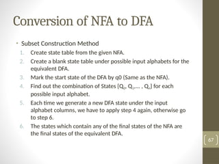
  • 67. Conversion of NFA to DFA • Subset Construction Method 1. Create state table from the given NFA. 2. Create a blank state table under possible input alphabets for the equivalent DFA. 3. Mark the start state of the DFA by q0 (Same as the NFA). 4. Find out the combination of States {Q0, Q1,... , Qn} for each possible input alphabet. 5. Each time we generate a new DFA state under the input alphabet columns, we have to apply step 4 again, otherwise go to step 6. 6. The states which contain any of the final states of the NFA are the final states of the equivalent DFA. 67
  • 70. Transition Diagram for the subset 70
  • 72. NFA  DFA State 0 1 →q0 q0 q1 q1 {q1, q2} q1 *q2 q2 {q1, q2} 72
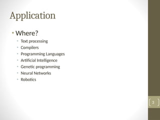
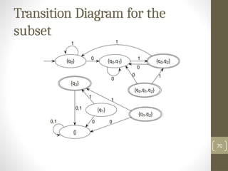
  • 73. Now we will obtain δ' transition for state q0. δ'([q0], 0) = [q0] δ'([q0], 1) = [q1] The δ' transition for state q1 is obtained as: δ'([q1], 0) = [q1, q2] (new state generated) δ'([q1], 1) = [q1] 73
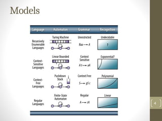
  • 74. Now we will obtain δ' transition on [q1, q2]. δ'([q1, q2], 0) = δ(q1, 0) ∪ δ(q2, 0) = {q1, q2} ∪ {q2} = [q1, q2] δ'([q1, q2], 1) = δ(q1, 1) ∪ δ(q2, 1) = {q1} ∪ {q1, q2} = {q1, q2} = [q1, q2] The state [q1, q2] is the final state as well because it contains a final state q2. 85
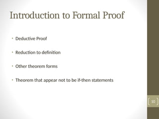
  • 75. The transition table for the constructed DFA will be: State 0 1 →[q0] [q0] [q1] [q1] [q1, q2] [q1] *[q1, q2] [q1, q2] [q1, q2] 86
  • 76. Conversion of - ε NFA to DFA • Modified subset construction 1. Find the ε-closure for the starting state of ε - NFA as a starting state of DFA. 2. Find the states for each input symbol that can be traversed from the present. That means the union of transition value and their closures for each state of NFA present in the current state of DFA. 3. If a new state is found, take it as current state and repeat step 2. 4. Repeat Step 2 and Step 3 until there is no new state present in the transition table of DFA. 5. Mark the states of DFA as a final state which contains the final state of ε-NFA. 87
  • 77. Example • Let us obtain ε-closure of each state. ε-closure {q0} = {q0, q1, q2} ε-closure {q1} = {q1} ε-closure {q2} = {q2} ε-closure {q3} = {q3} ε-closure {q4} = {q4} 77
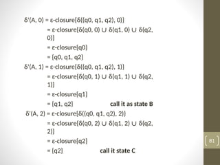
  • 78. •let ε-closure {q0} = {q0, q1, q2} be state A δ'(A, 0) = ε-closure {δ((q0, q1, q2), 0) } = ε-closure {δ(q0, 0) ∪ δ(q1, 0) ∪ δ(q2, 0) } = ε-closure {q3} = {q3} call it as state B. δ'(A, 1) = ε-closure {δ((q0, q1, q2), 1) } = ε-closure {δ((q0, 1) ∪ δ(q1, 1) ∪ δ(q2, 1)} = ε-closure {q3} = {q3} = B. 78
  • 79. δ'(B, 0) = ε-closure {δ(q3, 0) } = ϕ δ'(B, 1) = ε-closure {δ(q3, 1) } = ε-closure {q4} = {q4} i.e. state C δ'(C, 0) = ε-closure {δ(q4, 0) } = ϕ δ'(C, 1) = ε-closure {δ(q4, 1) } = ϕ 79
  • 80. ε-closure(q0) = {q0, q1, q2} ε-closure(q1) = {q1, q2} ε-closure(q2) = {q2} 80
  • 81. δ'(A, 0) = ε-closure{δ((q0, q1, q2), 0)} = ε-closure{δ(q0, 0) ∪ δ(q1, 0) ∪ δ(q2, 0)} = ε-closure{q0} = {q0, q1, q2} δ'(A, 1) = ε-closure{δ((q0, q1, q2), 1)} = ε-closure{δ(q0, 1) ∪ δ(q1, 1) ∪ δ(q2, 1)} = ε-closure{q1} = {q1, q2} call it as state B δ'(A, 2) = ε-closure{δ((q0, q1, q2), 2)} = ε-closure{δ(q0, 2) ∪ δ(q1, 2) ∪ δ(q2, 2)} = ε-closure{q2} = {q2} call it state C 81
  • 82. δ'(B, 0) = ε-closure{δ((q1, q2), 0)} = ε-closure{δ(q1, 0) ∪ δ(q2, 0)} = ε-closure{ϕ} = ϕ δ'(B, 1) = ε-closure{δ((q1, q2), 1)} = ε-closure{δ(q1, 1) ∪ δ(q2, 1)} = ε-closure{q1} = {q1, q2} i.e. state B itself δ'(B, 2) = ε-closure{δ((q1, q2), 2)} = ε-closure{δ(q1, 2) ∪ δ(q2, 2)} = ε-closure{q2} = {q2} i.e. state C 82
  • 83. δ'(C, 0) = ε-closure{δ(q2, 0)} = ε-closure{ϕ} = ϕ δ'(C, 1) = ε-closure{δ(q2, 1)} = ε-closure{ϕ} = ϕ δ'(C, 2) = ε-closure{δ(q2, 2)} = {q2} 83