SlideShare a Scribd company logo
Data Modeling Using the ER Model
Unit 2
III Semester BCA
Academic Year 2023-24
High level conceptual data models for DB design
Ø Database designer interviews prospective database user to understand and document their
data requirements
Ø Functional requirements - These user-defined operations include both retrievals and
update
Ø Create a conceptual schema for the database using a high level conceptual data model
Ø Users’ database requirements are illustrated briefly in the conceptual schema ( complete
descriptions of the entity types, relationships and constraints )
Ø From a high level data model, the conceptual schema is changed into the implementation
data model using a Commercial DBMS , mostly using relational or the object database
model
Internal storage structures, access paths, and file organizations are specified
High level conceptual data models for DB design
Parallel with these activities, application programs are designed and implemented as
database transactions corresponding to the high level transaction specifications.
The overall database design involves the following steps:
1) Identifying all the required files.
2) Identifying the fields of each of these files.
3) Identifying the primary key of each of these files.
4) Identifying the relationships between files.
High level conceptual data models for DB design
Let us consider an example database application called COMPANY database. The
COMPANY database keeps track of a company’s employees, departments and projects.
v The company is organized into departments each department has a unique name, a
unique number and a particular employee who manages the department.
v A department controls a number of project, each of which has a unique name, a unique
number each employee will have employee name, empid, address, salary, sex and date
of birth.
v An employee is assigned to one department but may work on several projects, which
are not necessarily controlled by the same department. Number of hours per week that
an employee works on each project is to be noted.
v Also each employee may have one or more dependents. These details are to be
maintained for insurance purposes. The dependent’s name, sex, birth date and
relationship to the employee are maintained.
Database Application -Example
Department: Dept no, Dept name, Dept location, Manager
Project : Proj no, Proj name
Employee : Emp id, Emp name, address, sex, salary, date of birth
Dependent : Dep name, sex, dob, relationship
Database Application -Example
E-R model
Ø describes data in terms of entities, relationships and attributes.
Entity:
Ø An entity is a thing in the real world with an independent existence.
Ø An entity may be an object with a physical existence such as person, a car, a building
or
May be an object with conceptual existence such as course, company or job.
Attribute:
Ø Property that describes an entity.
Examples:
STUDENT (Regno, Name, Age, Address)
EMPLOYEE(Id,Name, Dept,Salary)
COMPANY( Name, HQ, President)
E-R Model, Entity , Attributes
1. Simple Attribute
Ø is an atomic attribute that cannot be divided any further
Ø represents a single value.
Ø Example: In Employee" entity, "EmployeeID" is a simple
attribute
2. Composite Attribute
Ø attribute that can be divided into smaller sub-parts-each of which
represents a simpler attribute with its own meaning.
Ø Example: The "Address" attribute can be composed of sub-parts
like "Street," "City," and "Postal Code" in a "Customer" entity.
Attributes - Types
3. Derived Attribute
Ø attribute whose value can be derived from other attributes
within the database.
Ø Example: The "Age" of a person can be derived from their
"Date of Birth" in a "Person" entity.
4. Stored attribute
Ø The value of certain attributes that cannot be obtained or
derived from some other attributes are said to be stored
attributes.
Ø Example : Date of Birth" in a "Person" entity.
Attributes - Types
5. Multi-valued Attribute
Ø attribute can hold multiple values for a single entity.
Ø Example: In a "Book" entity, "Authors" can be a multi-valued
attribute because a book can have multiple authors.
Ø Two types:
ü Multi-valued Composite Attribute
ü Multi-valued Derived Attribute
Attributes - Types
a) Multi-valued Composite Attribute:
Ø combines the characteristics of both multi-valued and
composite attributes.
Ø Example: In a "Product" entity, "Features" can be a multi-
valued composite attribute with sub-parts like "Color," "Size,"
and "Weight."
b) Multi-valued Derived Attribute:
Ø combines the characteristics of multi-valued and derived
attributes.
Ø Example: In a "Sales" entity, "TotalSales" can be a multi-
valued derived attribute for a salesperson, representing the
total sales for different months.
Attributes - Types
6. Key Attribute
Ø used to uniquely identify instances of an entity within its entity
set.
Ø Example: "ISBN" can be a key attribute for a "Book" entity to
uniquely identify each book.
7.Single-valued Attribute
Ø holds a single value for each entity instance
Ø Example: "FirstName" and "LastName" are single-valued
attributes for a "Customer" entity.
Attributes - Types
8.Null Value Attribute
Ø For an entity ,if a particular attribute doesnot have any applicable
value then null value is assigned.
Null value can be assigned to the attribute in two cases.
1.A particular attribute is not applicable at all for the entity.
Example: For undergraduate students, the attribute degree is not
applicable at all. In that case a null value may be assigned to that
particular attribute.
2.The value of the attribute is not known, but it is applicable .
Example, if the age of a particular student is not known, then also
a null value can be assigned to it.
Attributes - Types
9. Complex Attribute:
Ø attribute has both composite and multi-valued components.
Ø Example: In a "University" entity, "Degrees" can be a complex
attribute with sub-parts like "Bachelor's," "Master's," and
"Ph.D.," and each of these can have multiple values for
different students.
Attributes - Types
Ø represents a category or class of objects with similar attributes, behaviors,
and characteristics
Ø defines a template for a group of entities that share common properties
Ø correspond to tables in a relational database, where each row in the table
represents an entity, and each column represents an attribute of that entity
type.
Ø depicted in ER diagrams as rectangles with the name of the entity type
written inside.
Ø Example: In a library database, you might have an "Author" entity type,
which represents all authors of books in the library. It would have
attributes like "AuthorID," "FirstName," and "LastName."
Entity Type???
Ø is a collection or set of entities of the same entity type
Ø represents the actual instances or objects of that entity type
Ø analogous to tables filled with data in a relational database. Each row in
an entity set corresponds to a specific entity instance.
Ø are the instances of an entity type that exist in the database at a given
time.
Ø In an ER diagram, an entity set is depicted as a set of labeled ovals
connected to the corresponding entity type by a straight line.
Ø Example: In the library database example, if "Author" is an entity type,
the "Author Entity Set" would contain individual author instances, such
as "Author 1: J.K. Rowling," "Author 2: George Orwell," and so on. Each
of these instances is part of the "Author Entity Set."
Entity Set???
Ø is an attribute of an entity type that is used to uniquely identify each entity
instance within that entity type.
Ø play a crucial role in ensuring data integrity and establishing relationships
between entities.
Ø Uniqueness: A key attribute must contain unique values for each entity instance
within the entity set
Ø Identification: Key attributes are used to identify individual entity instances
within the entity type.
Ø Primary Key: key attribute is also referred to as the "primary key" of the entity
type
Ø Relationships: Key attributes are often used as reference points in establishing
relationships between entities . i.e)the primary key of one table can be used as a
foreign key in another table to establish relationships between the two.
Ø Constraints: Used to enforce constraints, such as uniqueness constraints
Key Attribute???
Ø set of permissible values that an attribute can take
Ø used to define the range of valid values for attributes in a database schema
Ø They help to ensure data integrity and consistency by restricting the type and
range of data that can be stored in a particular attribute
Ø Data Validation: Value sets are used to validate data entered into attributes.
Ø Data Consistency: By limiting the values that an attribute can take, value sets
promote data consistency.
Ø Data Integrity: Value sets help maintain data integrity by preventing incorrect or
invalid data from being stored in attributes.
Ø Domain Constraints: Value sets can also include constraints( minimum and
maximum values, regular expressions, referential integrity constraints)
Ø Reuse: Domains can be defined once and reused for multiple attributes in the
same or different entities.
Ø Examples of Value Sets:Numeric Domain.Text Domain,Date Domain,Enumerated
Domain
Value sets of Attributes
Initial Conceptual Design of the COMPANY Database
There are four entity types for the company database namely department, project
employee and department with the following features.
1. Entity type: DEPARTMENT
Attributes: Name, Numbers, Locations, Manager and start date.
Key attributes: Name and Number
Multi-value attributes: Locations.
2. Entity Type: PROJECT
Attributes: Name, Number, Location, duration
Key attributes: Name, Number
3. Entity Type: EMPLOYEE
Attributes: Name, Sex, Address, Salary, Birthdate, Department.
Composite attributes: Address
4. Entity Type: DEPENDENT
Attributes: Employee, Dependent name, Sex, Birthdate, Relationship to the employee
Definition:
Ø is a meaningful association between two or more entities.
Ø represents how data is shared or linked between these entities.
Ø play a crucial role in defining the structure of a database and how different entities
interact with each other.
Ø Attributes: Relationships can have attributes that provide additional information
about the association itself. These attributes are often called "relationship
attributes" or "associative attributes."
Ø Role Names: Role names are used to specify the roles that each participating
entity plays in a relationship. Role names make the relationship more descriptive
and clarify the meaning of the connection between entities.
Relationship in ER Model
Cardinality:
Ø defines the number of instances of one entity that can be associated with the
number of instances of another entity.
One-to-One (1:1): Each instance of one entity is associated with exactly one instance
of another entity, and vice versa.
One-to-Many (1:N): Each instance of one entity is associated with zero, one, or
many instances of another entity, but each instance of the other entity is associated
with at most one instance of the first entity.
Many-to-One (N:1): The reverse of "One-to-Many," where each instance of one
entity is associated with at most one instance of another entity, but each instance of
the other entity can be associated with zero, one, or many instances of the first entity.
Many-to-Many (N:N): Each instance of one entity can be associated with zero, one,
or many instances of another entity, and vice versa.
Relationship in ER Model
Dependent and Independent Entities: In a relationship, one entity is often referred to
as the "dependent entity," and the other is the "independent entity." The dependent
entity relies on the independent entity for its existence.
Relationship Constraints: Constraints, such as referential integrity rules, can be
applied to relationships to enforce data consistency and integrity.
ER Diagrams: Relationships are typically represented in ER diagrams using diamond
shapes connecting the related entities.
The cardinality and role names are often indicated near the diamond shape.
Relationship in ER Model
Example:
Consider a database for a university. You might have entities like "Student" and
"Course." The relationship between them could be represented as follows:
Name: Enroll
Cardinality: Many-to-Many (since a student can enroll in multiple courses, and a
course can have multiple students)
Role Names: "Student" (for the student's role) and "Course" (for the course's role)
Attributes: An attribute might be "EnrollmentDate," which indicates when a student
enrolled in a particular course.
Relationship in ER Model
Degree of a relationship refers to the number of entity types (or entities)
that participate in that relationship.
Unary Relationship (Degree 1): In a unary relationship, an entity is
related to itself.
Example, you might use a unary relationship to model a "Supervises"
relationship between employees in an organization, where an employee can
supervise other employees.
Binary Relationship (Degree 2): A binary relationship involves two entity
types or entities.
Example: in a university database, you could have a binary relationship
between "Student" and "Course" to represent the fact that students enroll in
courses.
Degree of Relationship
Ternary Relationship (Degree 3): A ternary relationship involves three entity
types or entities.
Example, in a hospital database, you might have a ternary relationship
between "Doctor," "Patient," and "Diagnosis" to show which doctor diagnosed
a particular patient with a specific condition.
Degree of Relationship
Participation Constraints
1. Total Participation Constraints
Participation Constraints
2. Partial Participation Constraints
Attributes of Relationship Types
Relationship types can also have attributes, similar to those of entity types.
Weak Entity Types
Ø Entity types that do not have key attributes of their own are called weak entity types.
Ø Entities belonging to a weak entity type are identified by being related to specific entities
from another entity type in combination with some of their attribute values- identifying
or owner entity type and the relationship type - identifying relationship of the weak entity
type.
Ø A weak entity type always has a total participation constraint with respect to its
identifying relationship because a weak entity cannot be identified without an owner
entity.
E-R diagram
ØAn Entity Relationship Diagram( ERD)- shows the relationships
of a set of entities stored in a ER diagrams
Øexplains the logical structure of a database.
ØER based on three basic concepts: entities, attributes, and
relationships.
E-R diagram
E-R diagram- Symbols
Company Database- Description
Ø A company is organized into departments.
Ø Each department has a unique name and number and is headed by a specific
employee.
Ø Track this employee's start date. We started leading the department.
Ø Departments can have multiple locations.
Ø Departments manage multiple projects with unique names, numbers, and locations.
Ø Store each employee's name, social security number, address, salary, gender, and
date of birth.
Ø Employees are assigned to departments but work on some non-essential projects
managed by the same department.
Ø Track hours per Week on which employees work on all projects.
Ø Also track each line manager-employee.
Ø Want to track everyone's family Clerk for insurance purposes.
Ø Retains name, gender, date of birth, and all family members
E-R diagram
Entities and their Attributes
Ø Employee Entity : Attributes of Employee Entity are Name, Id, Address, Gender, Dob and Doj.
Id is Primary Key for Employee Entity.
Ø Department Entity : Attributes of Department Entity are D_no, Name and Location.
D_no is Primary Key for Department Entity.
Ø Project Entity : Attributes of Project Entity are P_No, Name and Location.
P_No is Primary Key for Project Entity.
Ø Dependent Entity : Attributes of Dependent Entity are D_name, Gender and relationship.
E-R diagram
Relationships:
Employees works in Departments – Many employee works in one Department but one employee can
not work in many departments.
Manager controls a Department – employee works under the manager of the Department and the
manager records the date of joining of employee in the department.
Department has many Projects – One department has many projects but one project can not come
under many departments.
Employee works on project –
One employee works on several projects and the number of hours worked by the employee on a
single project is recorded.
Employee has dependents –
Each Employee has dependents. Each dependent is dependent of only one employee.
E-R diagram-
Company
E-R diagram -Bank
Bank have Customer.
Banks are identified by a name, code, address of main office.
Banks have branches.
Branches are identified by a branch_no., branch_name, address.
Customers are identified by name, cust-id, phone number, address.
Customer can have one or more accounts.
Accounts are identified by account_no., acc_type, balance.
Customer can avail loans.
Loans are identified by loan_id, loan_type and amount.
Account and loans are related to bank’s branch.
E-R diagram -Bank
Entities and their Attributes :
Bank Entity : Attributes of Bank Entity are Bank Name, Code and Address.
Code is Primary Key for Bank Entity.
Customer Entity : Attributes of Customer Entity are Customer_id, Name, Phone
Number and Address.
Customer_id is Primary Key for Customer Entity.
Branch Entity : Attributes of Branch Entity are Branch_id, Name and Address.
Branch_id is Primary Key for Branch Entity.
Account Entity : Attributes of Account Entity are Account_number, Account_Type
and Balance.
Account_number is Primary Key for Account Entity.
Loan Entity : Attributes of Loan Entity are Loan_id, Loan_Type and Amount.
Loan_id is Primary Key for Loan Entity.
E-R diagram -Bank
Relationships are :
Bank has Branches => 1 : N
Branch maintain Accounts => 1 : N
Branch offer Loans => 1 : N
Account held by Customers => M : N
Loan availed by Customer => M : N
E-R diagram-
Bank
Record Storage and Primary file organization
Ø File is a collection of records. Using the primary key, we can access the
records.
Ø Type and frequency of access depends on the type of file organization used for
a given set of records.
Ø File organization is a logical relationship among various records-defines how
file records are mapped onto disk blocks.
Ø File organization is used to describe the way in which the records are stored in
terms of blocks, and the blocks are placed on the storage medium.
Ø Files of fixed length records are easier to implement than the files of variable
length records.
File organization - Objectives
Ø It contains an optimal selection of records - records can be selected as fast as
possible.
Ø To perform insert, delete or update transaction on the records ina quick and
easy way.
Ø Duplicate records cannot be induced as a result of insert, update or delete.
Ø With minimal cost of storage, records should be stored efficiently.
Disk - Hardware description
v The entire disk is divided into platters.
v Each platter consists of concentric circles called as tracks.
v These tracks are further divided into sectors which are
the smallest divisions in the disk.
v A cylinder is formed by combining the tracks at a given
radius of a disk pack.
v There exists a mechanical arm called as Read / Write
head.
v It is used to read from and write to the disk.
v Head has to reach at a particular track and then wait for
the rotation of the platter.
v The rotation causes the required sector of the track to
come under the head.
v Each platter has 2 surfaces- top and bottom and both the
surfaces are used to store the data.
v Each surface has its own read / write head.
Disk - Hardware description
The time taken by the disk to complete an I/O request is called as disk service time
or disk access time.
1. Seek Time :
Ø The time taken by the read / write head to reach the desired track is called as
seek time.
Ø It is the component which contributes the largest percentage of the disk service
time.
Ø The lower the seek time, the faster the I/O operation.
2. Rotational Latency:
Ø The time taken by the desired sector to come under the read / write head is
called as rotational latency.
Ø It depends on the rotation speed of the spindle.
Disk - Hardware description
3. Data Transfer Rate:
Ø The amount of data that passes under the read / write head in a given amount
of time is called as data transfer rate.
Ø The time taken to transfer the data is called as transfer time.
Ø It depends on the following factors-
Ø Number of bytes to be transferred
Ø Rotation speed of the disk
Ø Density of the track
Ø Speed of the electronics that connects the disk to the computer
Disk - Hardware description
4. Controller Overhead:
Ø The overhead imposed by the disk controller is called as controller
overhead.
Disk controller is a device that manages the disk.
5. Queuing Delay:
Ø The time spent waiting for the disk to become free is called as queuing
delay.
Disk - Hardware description
Disk access time :
Disk access time = Seek time + Rotational delay + Transfer time + Controller
overhead + Queuing delay
Disk - Hardware description
Disk access time :
Disk access time = Seek time + Rotational delay + Transfer time + Controller
overhead + Queuing delay
Why RAID?
It is a technique that combines multiple disk drives into a logical unit (RAID
set) and provides protection, performance, or both.
RAID
RAID can be implemented by
• Software RAID implementation
4 Uses host-based software to provide RAID functionality
• Hardware RAID Implementation
4 Uses a specialized hardware controller installed either on a host or on an
array
RAID Techniques
Three key techniques used for RAID are:
Ø Striping
Ø Mirroring
Ø Parity
RAID Techniques - Striping
RAID Techniques - Mirroring
RAID Techniques - Parity
RAID Levels
• Commonly used RAID levels are:
4 RAID 0 – Striped set with no fault tolerance
4 RAID 1 – Disk mirroring
4 RAID 1 + 0 – Nested RAID
4 RAID 3 – Striped set with parallel access and dedicated parity disk
4 RAID 5 – Striped set with independent disk access and a
distributed parity
4 RAID 6 – Striped set with independent disk access and dual
distributed parity
RAID Levels - RAID 0
RAID Levels - RAID 1
RAID Levels - RAID 1 + 0
RAID Levels - RAID 3
RAID Levels - RAID 5
RAID Levels - RAID 6
Buffering of Blocks
Buffering - temporary storage of data in a buffer, or a small, fixed-sized area in
memory, while it is being moved from one place to another.
Two types of buffering
Input buffering - temporary storage of data that is being received from an external
source, such as a file on a hard drive or data being transmitted over a network.
Output buffering - temporary storage of data that is being sent to an external
destination, such as a printer or a file on a hard drive.
In DBMS buffering is used to temporarily store data as it is being written to or read
from a database. For example, when you update a record in a database, the changes
may be temporarily stored in a buffer before they are written to the database.
Buffering of Blocks -Why?
ü When blocks are transferred to memory, they are
held in buffers.
ü If several blocks need to be transferred from the
disk to main memory, several buffers can be
reserved in main memory to speed up the transfer.
ü While one buffer is being read/written, the CPU
can process data in the other buffer which is
possible because the block transfer is controlled
by an independent disk I/O processor, which can
transfer data blocks between main memory and
the disk, independent of, and in parallel to the
CPU processing data already stored in memory.
ü Two ways this processing : interleaved fashion or
in a parallel fashion.
Buffering of Blocks - Benefits
Improved performance − Buffering allows data to be transferred more efficiently,
which can improve the overall performance of the system.
Error detection and recovery − By transferring data in smaller blocks, it is easier to
detect and recover from errors that may occur during the transfer process.
Reduced risk of data loss − Buffering can help to prevent data loss by temporarily
storing data in a buffer before it is written to a permanent storage location.
Greater flexibility − Buffering allows data to be transferred asynchronously, which
means that the data can be transferred at a time that is convenient for the system
rather than all at once.
How to Buffer Blocks
Fixed-size block buffering
Ø Buffer is divided into a fixed number of blocks,of a fixed size.
Ø When data is written to the buffer, it is divided into blocks of the specified size
and written to the appropriate block in the buffer.
Ø Simple to implement, but it can be inefficient if the block size does not match the
size of the data being written.
Dynamic block buffering
Ø The size of the blocks in the buffer is not fixed and the buffer is divided into a
series of linked blocks, and the size of each block is determined by the amount of
data that it contains.
Ø Flexible than fixed-size block buffering, but it can be more complex to implement.
How to Buffer Blocks
Circular block buffering
Ø Buffer is treated as a circular buffer, with data being written to the buffer and then
overwriting the oldest data as the buffer becomes full.
Ø Simple to implement and can be efficient, but it can lead to data loss if the data is
not processed quickly enough.
Double Buffering
Ø Used in database management systems to enhance data processing and transmission.
Two buffers are used, one of which is actively used for input and output activities
while the second buffer gathers data for processing.
Ø The buffers are switched when processing is finished which enables smooth data
flow and reduces wait times.
Double Buffering - Implementation
1. Two buffers must be created and initialised suitably in
accordance with the needs of the programme.
2. Buffer manager is in charge of assigning space in the
buffers for data storage after they have been set up. The
buffer manager controls internal tasks and makes sure
the buffers are used effectively.
3. It is possible to write to one buffer while reading from
another, enabling smooth multitasking and better
performance.
4. Buffers are switched when data processing is finished,
ensuring a smooth transition between the old and new
data sets.
Record Blocking
Types of Record Blocking
1.Fixed blocking
2. Variable-length spanned blocking
3. Variable-length unspanned blocking
Records are the logical unit of a file and blocks are units of I/O with secondary
storage.
For I/O the records must be organized as blocks.
Blocking is a process of grouping similar records into blocks that the operating
system component explores exhaustively.
Larger blocks reduce the I/O transfer time but requires larger I/O buffers
In record blocking, the records are grouped into blocks by shared properties that
are indicators of duplication.
Record Blocking - Types
3. Variable-length unspanned blocking
1. Fixed blocking
Ø Record lengths are fixed
Ø Prescribed number of records stored in a block
Ø Internal fragmentation is stored in a block.
Ø Used for sequential files with fixed-length records
When the block size is larger than the record size, the block will contain multiple records.
Let B be the Block size and R:be the Fixed length record size in bytes.
If B (size of the block) is greater that R (size of the fixed length record) then we know that
we can fit B/R records per block. This is called the blocking factor (bfr).
Blocking factor:
bfr = ëB/Rû
Unused Block Space = B – (bfr * R) bytes
Blocking factor
Record Blocking - Types
2. Variable-length spanned blocking
Ø Record sizes aren’t same, Variable-length records packed into blocks with no unused space.
Some records may divide into two blocks,where a pointer passes from one block to another
block. So, the Pointers are used to span block unused space.
Ø It is efficient in length and efficiency of storage.
Ø It doesn’t limit record size, but it is more complicated to implement. So, the files are more
difficult to update
Record Blocking - Types
3. Variable-length unspanned blocking
Ø Records are variable in length, but the records doesnot span between blocks.
Ø In this method, the wasted area is a serious problem, because of the inability to
use the remainder of a block, if the next record is larger than the remaining
unused space. These blocking methods results in wasted space and limit record
size to the size of the block.
File Allocation-Methods
v Define how the files are stored in the disk blocks
v Aims at Efficient disk space utilization and Fast access to the file blocks.
1. Contiguous Allocation
Each file occupies a contiguous set of blocks on the disk. i.e) if a file requires
n blocks and is given a block b as the starting location, then the blocks
assigned to the file will be: b, b+1, b+2,……b+n-1.
Given the starting block address and the length of the file (in terms of blocks
required), we can determine the blocks occupied by the file.
The directory entry for a file with contiguous allocation contains
Ø Address of starting block
Ø Length of the allocated portion.
File Allocation-Methods
1. Contiguous Allocation
File Allocation-Methods
2. Linked List Allocation
Each file is a linked list of disk blocks which need not be contiguous. The disk blocks can
be scattered anywhere on the disk.
The directory entry contains a pointer to the starting and the ending file block. Each block
contains a pointer to the next block occupied by the file.
The file ‘jeep’ in following image shows how the blocks are randomly distributed. The last
block (25) contains -1 indicating a null pointer and does not point to any other block.
File Allocation-Methods
3. Indexed Allocation
Ø A special block known as the Index block contains the pointers to all the
blocks occupied by a file.
Ø Each file has its own index block. The ith entry in the index block contains
the disk address of the ith file block.
File Operations
Operations on database files can be broadly classified into two categories
Ø Update Operations -insertion, deletion, or update
Ø Retrieval Operations -locate certain records so their field values can be examined
and processed.
Ø Record-at –a time operation or Set-at-a-time operations
File Processing happens as:
Ø Open − A file can be opened in one of the two modes, read mode or write mode
Ø Locate − Every file has a file pointer, which tells the current position where the data
is to be read or written.
Ø Read − By default, when files are opened in read mode, the file pointer points to the
beginning of the file.
Ø Write − User can select to open a file in write mode, which enables them to edit its
contents. It can be deletion, insertion, or modification.
Ø Close − removes all the locks ,saves the data to the secondary storage media and
Ø releases all the buffers and file handlers associated with the file.
File Organisations
A file organisation refers to the the way records and blocks are placed on the storage
medium and linked. Some types of File Organizations are :
1. Sequential File Organization :
File is stored one after another in a sequential manner.
1. Pile File Method - store the records in a sequence i.e. one after the other in the order
in which they are inserted into the tables-new one at end
2. Sorted File Method - new record is always inserted in a sorted (ascending or
descending) manner. The sorting of records may be based on any primary key or any
other key.
File Organisations
2. Heap File Organization
Ø records are inserted at the end of the file, into the data blocks.
Ø No Sorting or Ordering is required in this method.
Ø If a data block is full, the new record is stored in some other block, Here the other
data block need not be the very next data block, but it can be any block in the
memory.
Ø It is the responsibility of DBMS to store and manage the new records.
File Organisations
3. Hash File Organization :
Ø Also called a direct file organisation.
Ø For storing the records a hash function is calculated on some fields of the record,
which provides the address of the block to store the record. Any type of
mathematical function can be used as a hash function
Ø Hashing uses a hash function, h, that is applied to the hash field value of a record
and gives the address of the disk block in which the record is stored.
Internal Hashing
Ø For internal files, hashing is typically implemented as a hash table through the use
of an array of records.
Ø Suppose that the array index range is from 0 to M – 1, then we have M slots whose
addresses correspond to the array indexes.
Ø We choose a hash function that transforms the hash field value into an integer
between 0 and M − 1.
Ø One common hash function is the h(K) = K mod M function, which returns the
remainder of an integer hash field value K after division by M; this value is then
used for the record address.
Ø Noninteger hash field values can be transformed into integers before the mod
function is applied.
Internal Hashing
Internal Hashing
Ø Folding involves applying an arithmetic function such as addition or logical function
such as exclusive or (Xor) to different portions of the hash field value to calculate
the hash address.
Ø Another technique involves picking some digits of the hash field value (ie. Third,
fifth, eighth digits) to form the hash address.
Problem:
Ø hashing functions is that they don’t guarantee that distinct values will hash to
distinct addresses- Many values can hash to the same address
Ø This is because the hash field space is much larger than the address space .
Collision Resolution Mechanisms
Open Addressing/Linear Probing :
Ø if the hash address is occupied, the program checks the next positions in order
until an empty address is found.
Chaining :
Ø Overflow locations are used, by extending the array with overflow positions.
Ø Each record location has a pointer field, and if the hash address is occupied,
the collision is resolved by placing the new record in an unused overflow
location, and setting the pointer of the occupied hash address location to the
address of the overflow location.
Ø A linked list of the overflow records for each hash address is maintained.
Multiple hashing :
Ø If the first hash function results in a collision, a second hash function is
applied. If there is a collision after the second hash function, either a third
hash function is applied, or open addressing is used.
External Hashing
Ø Hashing for disk files is called external hashing.
Ø The target address space is made up of buckets (blocks).A bucket can be either
one disk block, or multiple contiguous blocks.
Ø Each bucket holds multiple records.
Ø The hashing function maps a key into a relative bucket number, rather than
assign an absolute block address to the bucket.
Ø A table maintained in the file header converts the bucket number into the
corresponding block address
Ø the collision problem is less severe, because many records can hash to the same
bucket. and if a bucket becomes full and new records hashing to a full bucket,
collision resolving mechanisms again must be used.
Ø every bucket maintains a pointer to a linked list of overflow records for that
bucket.
External Hashing
Ø This hashing scheme is called static hashing because a fixed number of
buckets, M, is allocated for the address space. If m is the maximum number
of records that can fit into a bucket, the total capacity allocated for all
buckets is (M * m). If there are significantly fewer than (M * m) records,
then there is a lot of unused record space.And if there are more than (M*m)
records numerous collisions will result, and performance will be affected
because of the long lists of overflow records.
Ø Searching for a record when using external hashing is expensive if the
search field is not the hash field.
Ø Record deletion can be implemented by removing the record from its bucket.
If the bucket has an overflow chain, the overflow records can be moved into
the bucket to replace the deleted record.
External Hashing
External Hashing -Dynamic File Expansion
Ø In static hashing is that address space is fixedand indynamic file
organizations based on hashing allow the number of buckets to vary
dynamically with only localised reorganization.
External Hashing-Dynamic File Expansion
Extendible Hashing
Ø based on binary representation of a number.
Ø Apply a hashing function to a non negative integer, and represent the result
as a binary number- a string of bits -which is called the hash value of a
record.
Ø Records are distributed among buckets based on the values of the leading
bits in their hash values.
Ø a directory of 2d bucket addresses in maintained, d is the global depth of
the directory.
Ø The integer value corresponding to the first d bits of a hash value is used as
an index to the array to determine a directory entry, and the address in the
directory entry determines the bucket in which the corresponding records
are stored.
External Hashing - Dynamic File Expansion
Extendible Hashing
Ø A local depth, d1 stored with each bucket specifies the number of bits on
which the bucket contents are based.
Ø The value d can be increased or decreased by one at a time, doubling or
halving the number of entries in the directory.
External Hashing - Dynamic File Expansion
Linear Hashing
Ø allows a hash file to expand and shrink its number of buckets dynamically
without needing a directory.
Ø The file starts with M buckets, numbered 0 to M-1, and uses the initial hash
function h(K)= K mod M. Overflow because of collisions is needed, and
can be handled using an overflow chain for each bucket.
Ø When a collision leads to an overflow record in ANY file bucket, the first
bucket is split into two buckets, the original bucket 0, and a new bucket M
at the end of the file. The records in bucket 0 are distributed between the
two buckets based on a different hashing function, hi+1(K) = K mod M.
File Organisations
2. Heap File Organization
records are inserted at the end of the file, into the data blocks.
No Sorting or Ordering is required in this method.
If a data block is full, the new record is stored in some other block, Here the other data
block need not be the very next data block, but it can be any block in the memory.
It is the responsibility of DBMS to store and manage the new records.
THANK YOU

More Related Content

Similar to Unit 2-Data Modeling.pdf (20)

PPTX
Fundamentals of database system - Data Modeling Using the Entity-Relationshi...
Mustafa Kamel Mohammadi
 
PPTX
Introduction of Database Design and Development
Er. Nawaraj Bhandari
 
PDF
Database Systems - Entity Relationship Modeling (Chapter 4/2)
Vidyasagar Mundroy
 
PDF
ER diagram is created based on three principal components: entities, attribut...
athuathul507
 
PPT
Data modeling using the entity relationship model
Jafar Nesargi
 
PPT
database1
Monika Sharma
 
PPTX
dbms ppt parul university dbms course for
VaibhavSrivastav52
 
PDF
Advance database system(part 4)
Abdullah Khosa
 
PPTX
Database part3-
Taymoor Nazmy
 
PPT
Chapter3
Jafar Nesargi
 
PPT
Chapter3
Jafar Nesargi
 
PPTX
ER modeling
Dabbal Singh Mahara
 
PPTX
DATA MODEL PRESENTATION UNIT I-BCA I.pptx
JasmineMichael1
 
PPT
Data modelingpresentation
fikirabc
 
PDF
Database Design and the ER Model, Indexing and Hashing
Prabu U
 
PPTX
ER Modeling and Introduction to RDBMS
Rubal Sagwal
 
PPT
Chapter03 database system in computer.ppt
ubaidullah75790
 
PPT
Modern Database Management: Principles, Practices, and Applications
usarwar382
 
PPTX
UNIT 1 INTRODUCTION TO DBMS, ER DIAGRAM, RELATION
Bhakti Pawar
 
PPTX
Database week 5 lecture includes spexiafix
tasleemasad33
 
Fundamentals of database system - Data Modeling Using the Entity-Relationshi...
Mustafa Kamel Mohammadi
 
Introduction of Database Design and Development
Er. Nawaraj Bhandari
 
Database Systems - Entity Relationship Modeling (Chapter 4/2)
Vidyasagar Mundroy
 
ER diagram is created based on three principal components: entities, attribut...
athuathul507
 
Data modeling using the entity relationship model
Jafar Nesargi
 
database1
Monika Sharma
 
dbms ppt parul university dbms course for
VaibhavSrivastav52
 
Advance database system(part 4)
Abdullah Khosa
 
Database part3-
Taymoor Nazmy
 
Chapter3
Jafar Nesargi
 
Chapter3
Jafar Nesargi
 
ER modeling
Dabbal Singh Mahara
 
DATA MODEL PRESENTATION UNIT I-BCA I.pptx
JasmineMichael1
 
Data modelingpresentation
fikirabc
 
Database Design and the ER Model, Indexing and Hashing
Prabu U
 
ER Modeling and Introduction to RDBMS
Rubal Sagwal
 
Chapter03 database system in computer.ppt
ubaidullah75790
 
Modern Database Management: Principles, Practices, and Applications
usarwar382
 
UNIT 1 INTRODUCTION TO DBMS, ER DIAGRAM, RELATION
Bhakti Pawar
 
Database week 5 lecture includes spexiafix
tasleemasad33
 

More from MaryJacob24 (20)

PDF
Evaluation of Postfix Expression-Concept and Example
MaryJacob24
 
PDF
Huffman Encoding Algorithm - Concepts and Example
MaryJacob24
 
PDF
Introduction to Essentials of Virtualization
MaryJacob24
 
PDF
Structure in C Programming- Basic Concepts
MaryJacob24
 
PDF
Union in C Programming Language-Basic Concepts
MaryJacob24
 
PDF
Unit 1-Introduction to Data Structures-BCA.pdf
MaryJacob24
 
PDF
C Operators and Control Structures.pdf
MaryJacob24
 
PDF
Unit 4- Dynamic Programming.pdf
MaryJacob24
 
PPTX
Unit 3- Greedy Method.pptx
MaryJacob24
 
PDF
tree traversals.pdf
MaryJacob24
 
PDF
Linked List-Types.pdf
MaryJacob24
 
PDF
Unit 5- Cloud Applications.pdf
MaryJacob24
 
PDF
Simplification of Circuits.pdf
MaryJacob24
 
PDF
2 bit comparator, 4 1 Multiplexer, 1 4 Demultiplexer, Flip Flops and Register...
MaryJacob24
 
PDF
Algorithm-Introduction ,Characterestics & Control Structures.pdf
MaryJacob24
 
PDF
Data Structures & Recursion-Introduction.pdf
MaryJacob24
 
PDF
quick sort.pdf
MaryJacob24
 
PDF
Unit 3 - Greedy Method
MaryJacob24
 
PDF
Unit 3 greedy method
MaryJacob24
 
PDF
Graph Traversals
MaryJacob24
 
Evaluation of Postfix Expression-Concept and Example
MaryJacob24
 
Huffman Encoding Algorithm - Concepts and Example
MaryJacob24
 
Introduction to Essentials of Virtualization
MaryJacob24
 
Structure in C Programming- Basic Concepts
MaryJacob24
 
Union in C Programming Language-Basic Concepts
MaryJacob24
 
Unit 1-Introduction to Data Structures-BCA.pdf
MaryJacob24
 
C Operators and Control Structures.pdf
MaryJacob24
 
Unit 4- Dynamic Programming.pdf
MaryJacob24
 
Unit 3- Greedy Method.pptx
MaryJacob24
 
tree traversals.pdf
MaryJacob24
 
Linked List-Types.pdf
MaryJacob24
 
Unit 5- Cloud Applications.pdf
MaryJacob24
 
Simplification of Circuits.pdf
MaryJacob24
 
2 bit comparator, 4 1 Multiplexer, 1 4 Demultiplexer, Flip Flops and Register...
MaryJacob24
 
Algorithm-Introduction ,Characterestics & Control Structures.pdf
MaryJacob24
 
Data Structures & Recursion-Introduction.pdf
MaryJacob24
 
quick sort.pdf
MaryJacob24
 
Unit 3 - Greedy Method
MaryJacob24
 
Unit 3 greedy method
MaryJacob24
 
Graph Traversals
MaryJacob24
 
Ad

Recently uploaded (20)

PDF
Reconstruct, Restore, Reimagine: New Perspectives on Stoke Newington’s Histor...
History of Stoke Newington
 
PDF
Dimensions of Societal Planning in Commonism
StefanMz
 
PDF
0725.WHITEPAPER-UNIQUEWAYSOFPROTOTYPINGANDUXNOW.pdf
Thomas GIRARD, MA, CDP
 
PDF
community health nursing question paper 2.pdf
Prince kumar
 
PDF
Biological Bilingual Glossary Hindi and English Medium
World of Wisdom
 
PPTX
ASRB NET 2023 PREVIOUS YEAR QUESTION PAPER GENETICS AND PLANT BREEDING BY SAT...
Krashi Coaching
 
PPTX
Unit 2 COMMERCIAL BANKING, Corporate banking.pptx
AnubalaSuresh1
 
PDF
LAW OF CONTRACT ( 5 YEAR LLB & UNITARY LLB)- MODULE-3 - LEARN THROUGH PICTURE
APARNA T SHAIL KUMAR
 
PDF
Stokey: A Jewish Village by Rachel Kolsky
History of Stoke Newington
 
PDF
Chapter-V-DED-Entrepreneurship: Institutions Facilitating Entrepreneurship
Dayanand Huded
 
PPTX
Stereochemistry-Optical Isomerism in organic compoundsptx
Tarannum Nadaf-Mansuri
 
PDF
The History of Phone Numbers in Stoke Newington by Billy Thomas
History of Stoke Newington
 
PDF
Isharyanti-2025-Cross Language Communication in Indonesian Language
Neny Isharyanti
 
PPTX
Neurodivergent Friendly Schools - Slides from training session
Pooky Knightsmith
 
PDF
CONCURSO DE POESIA “POETUFAS – PASSOS SUAVES PELO VERSO.pdf
Colégio Santa Teresinha
 
PPTX
How to Create a PDF Report in Odoo 18 - Odoo Slides
Celine George
 
PDF
QNL June Edition hosted by Pragya the official Quiz Club of the University of...
Pragya - UEM Kolkata Quiz Club
 
PDF
Generative AI: it's STILL not a robot (CIJ Summer 2025)
Paul Bradshaw
 
PPTX
CATEGORIES OF NURSING PERSONNEL: HOSPITAL & COLLEGE
PRADEEP ABOTHU
 
PDF
Knee Extensor Mechanism Injuries - Orthopedic Radiologic Imaging
Sean M. Fox
 
Reconstruct, Restore, Reimagine: New Perspectives on Stoke Newington’s Histor...
History of Stoke Newington
 
Dimensions of Societal Planning in Commonism
StefanMz
 
0725.WHITEPAPER-UNIQUEWAYSOFPROTOTYPINGANDUXNOW.pdf
Thomas GIRARD, MA, CDP
 
community health nursing question paper 2.pdf
Prince kumar
 
Biological Bilingual Glossary Hindi and English Medium
World of Wisdom
 
ASRB NET 2023 PREVIOUS YEAR QUESTION PAPER GENETICS AND PLANT BREEDING BY SAT...
Krashi Coaching
 
Unit 2 COMMERCIAL BANKING, Corporate banking.pptx
AnubalaSuresh1
 
LAW OF CONTRACT ( 5 YEAR LLB & UNITARY LLB)- MODULE-3 - LEARN THROUGH PICTURE
APARNA T SHAIL KUMAR
 
Stokey: A Jewish Village by Rachel Kolsky
History of Stoke Newington
 
Chapter-V-DED-Entrepreneurship: Institutions Facilitating Entrepreneurship
Dayanand Huded
 
Stereochemistry-Optical Isomerism in organic compoundsptx
Tarannum Nadaf-Mansuri
 
The History of Phone Numbers in Stoke Newington by Billy Thomas
History of Stoke Newington
 
Isharyanti-2025-Cross Language Communication in Indonesian Language
Neny Isharyanti
 
Neurodivergent Friendly Schools - Slides from training session
Pooky Knightsmith
 
CONCURSO DE POESIA “POETUFAS – PASSOS SUAVES PELO VERSO.pdf
Colégio Santa Teresinha
 
How to Create a PDF Report in Odoo 18 - Odoo Slides
Celine George
 
QNL June Edition hosted by Pragya the official Quiz Club of the University of...
Pragya - UEM Kolkata Quiz Club
 
Generative AI: it's STILL not a robot (CIJ Summer 2025)
Paul Bradshaw
 
CATEGORIES OF NURSING PERSONNEL: HOSPITAL & COLLEGE
PRADEEP ABOTHU
 
Knee Extensor Mechanism Injuries - Orthopedic Radiologic Imaging
Sean M. Fox
 
Ad

Unit 2-Data Modeling.pdf

  • 1. Data Modeling Using the ER Model Unit 2 III Semester BCA Academic Year 2023-24
  • 2. High level conceptual data models for DB design
  • 3. Ø Database designer interviews prospective database user to understand and document their data requirements Ø Functional requirements - These user-defined operations include both retrievals and update Ø Create a conceptual schema for the database using a high level conceptual data model Ø Users’ database requirements are illustrated briefly in the conceptual schema ( complete descriptions of the entity types, relationships and constraints ) Ø From a high level data model, the conceptual schema is changed into the implementation data model using a Commercial DBMS , mostly using relational or the object database model Internal storage structures, access paths, and file organizations are specified High level conceptual data models for DB design
  • 4. Parallel with these activities, application programs are designed and implemented as database transactions corresponding to the high level transaction specifications. The overall database design involves the following steps: 1) Identifying all the required files. 2) Identifying the fields of each of these files. 3) Identifying the primary key of each of these files. 4) Identifying the relationships between files. High level conceptual data models for DB design
  • 5. Let us consider an example database application called COMPANY database. The COMPANY database keeps track of a company’s employees, departments and projects. v The company is organized into departments each department has a unique name, a unique number and a particular employee who manages the department. v A department controls a number of project, each of which has a unique name, a unique number each employee will have employee name, empid, address, salary, sex and date of birth. v An employee is assigned to one department but may work on several projects, which are not necessarily controlled by the same department. Number of hours per week that an employee works on each project is to be noted. v Also each employee may have one or more dependents. These details are to be maintained for insurance purposes. The dependent’s name, sex, birth date and relationship to the employee are maintained. Database Application -Example
  • 6. Department: Dept no, Dept name, Dept location, Manager Project : Proj no, Proj name Employee : Emp id, Emp name, address, sex, salary, date of birth Dependent : Dep name, sex, dob, relationship Database Application -Example
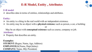
  • 7. E-R model Ø describes data in terms of entities, relationships and attributes. Entity: Ø An entity is a thing in the real world with an independent existence. Ø An entity may be an object with a physical existence such as person, a car, a building or May be an object with conceptual existence such as course, company or job. Attribute: Ø Property that describes an entity. Examples: STUDENT (Regno, Name, Age, Address) EMPLOYEE(Id,Name, Dept,Salary) COMPANY( Name, HQ, President) E-R Model, Entity , Attributes
  • 8. 1. Simple Attribute Ø is an atomic attribute that cannot be divided any further Ø represents a single value. Ø Example: In Employee" entity, "EmployeeID" is a simple attribute 2. Composite Attribute Ø attribute that can be divided into smaller sub-parts-each of which represents a simpler attribute with its own meaning. Ø Example: The "Address" attribute can be composed of sub-parts like "Street," "City," and "Postal Code" in a "Customer" entity. Attributes - Types
  • 9. 3. Derived Attribute Ø attribute whose value can be derived from other attributes within the database. Ø Example: The "Age" of a person can be derived from their "Date of Birth" in a "Person" entity. 4. Stored attribute Ø The value of certain attributes that cannot be obtained or derived from some other attributes are said to be stored attributes. Ø Example : Date of Birth" in a "Person" entity. Attributes - Types
  • 10. 5. Multi-valued Attribute Ø attribute can hold multiple values for a single entity. Ø Example: In a "Book" entity, "Authors" can be a multi-valued attribute because a book can have multiple authors. Ø Two types: ü Multi-valued Composite Attribute ü Multi-valued Derived Attribute Attributes - Types
  • 11. a) Multi-valued Composite Attribute: Ø combines the characteristics of both multi-valued and composite attributes. Ø Example: In a "Product" entity, "Features" can be a multi- valued composite attribute with sub-parts like "Color," "Size," and "Weight." b) Multi-valued Derived Attribute: Ø combines the characteristics of multi-valued and derived attributes. Ø Example: In a "Sales" entity, "TotalSales" can be a multi- valued derived attribute for a salesperson, representing the total sales for different months. Attributes - Types
  • 12. 6. Key Attribute Ø used to uniquely identify instances of an entity within its entity set. Ø Example: "ISBN" can be a key attribute for a "Book" entity to uniquely identify each book. 7.Single-valued Attribute Ø holds a single value for each entity instance Ø Example: "FirstName" and "LastName" are single-valued attributes for a "Customer" entity. Attributes - Types
  • 13. 8.Null Value Attribute Ø For an entity ,if a particular attribute doesnot have any applicable value then null value is assigned. Null value can be assigned to the attribute in two cases. 1.A particular attribute is not applicable at all for the entity. Example: For undergraduate students, the attribute degree is not applicable at all. In that case a null value may be assigned to that particular attribute. 2.The value of the attribute is not known, but it is applicable . Example, if the age of a particular student is not known, then also a null value can be assigned to it. Attributes - Types
  • 14. 9. Complex Attribute: Ø attribute has both composite and multi-valued components. Ø Example: In a "University" entity, "Degrees" can be a complex attribute with sub-parts like "Bachelor's," "Master's," and "Ph.D.," and each of these can have multiple values for different students. Attributes - Types
  • 15. Ø represents a category or class of objects with similar attributes, behaviors, and characteristics Ø defines a template for a group of entities that share common properties Ø correspond to tables in a relational database, where each row in the table represents an entity, and each column represents an attribute of that entity type. Ø depicted in ER diagrams as rectangles with the name of the entity type written inside. Ø Example: In a library database, you might have an "Author" entity type, which represents all authors of books in the library. It would have attributes like "AuthorID," "FirstName," and "LastName." Entity Type???
  • 16. Ø is a collection or set of entities of the same entity type Ø represents the actual instances or objects of that entity type Ø analogous to tables filled with data in a relational database. Each row in an entity set corresponds to a specific entity instance. Ø are the instances of an entity type that exist in the database at a given time. Ø In an ER diagram, an entity set is depicted as a set of labeled ovals connected to the corresponding entity type by a straight line. Ø Example: In the library database example, if "Author" is an entity type, the "Author Entity Set" would contain individual author instances, such as "Author 1: J.K. Rowling," "Author 2: George Orwell," and so on. Each of these instances is part of the "Author Entity Set." Entity Set???
  • 17. Ø is an attribute of an entity type that is used to uniquely identify each entity instance within that entity type. Ø play a crucial role in ensuring data integrity and establishing relationships between entities. Ø Uniqueness: A key attribute must contain unique values for each entity instance within the entity set Ø Identification: Key attributes are used to identify individual entity instances within the entity type. Ø Primary Key: key attribute is also referred to as the "primary key" of the entity type Ø Relationships: Key attributes are often used as reference points in establishing relationships between entities . i.e)the primary key of one table can be used as a foreign key in another table to establish relationships between the two. Ø Constraints: Used to enforce constraints, such as uniqueness constraints Key Attribute???
  • 18. Ø set of permissible values that an attribute can take Ø used to define the range of valid values for attributes in a database schema Ø They help to ensure data integrity and consistency by restricting the type and range of data that can be stored in a particular attribute Ø Data Validation: Value sets are used to validate data entered into attributes. Ø Data Consistency: By limiting the values that an attribute can take, value sets promote data consistency. Ø Data Integrity: Value sets help maintain data integrity by preventing incorrect or invalid data from being stored in attributes. Ø Domain Constraints: Value sets can also include constraints( minimum and maximum values, regular expressions, referential integrity constraints) Ø Reuse: Domains can be defined once and reused for multiple attributes in the same or different entities. Ø Examples of Value Sets:Numeric Domain.Text Domain,Date Domain,Enumerated Domain Value sets of Attributes
  • 19. Initial Conceptual Design of the COMPANY Database There are four entity types for the company database namely department, project employee and department with the following features. 1. Entity type: DEPARTMENT Attributes: Name, Numbers, Locations, Manager and start date. Key attributes: Name and Number Multi-value attributes: Locations. 2. Entity Type: PROJECT Attributes: Name, Number, Location, duration Key attributes: Name, Number 3. Entity Type: EMPLOYEE Attributes: Name, Sex, Address, Salary, Birthdate, Department. Composite attributes: Address 4. Entity Type: DEPENDENT Attributes: Employee, Dependent name, Sex, Birthdate, Relationship to the employee
  • 20. Definition: Ø is a meaningful association between two or more entities. Ø represents how data is shared or linked between these entities. Ø play a crucial role in defining the structure of a database and how different entities interact with each other. Ø Attributes: Relationships can have attributes that provide additional information about the association itself. These attributes are often called "relationship attributes" or "associative attributes." Ø Role Names: Role names are used to specify the roles that each participating entity plays in a relationship. Role names make the relationship more descriptive and clarify the meaning of the connection between entities. Relationship in ER Model
  • 21. Cardinality: Ø defines the number of instances of one entity that can be associated with the number of instances of another entity. One-to-One (1:1): Each instance of one entity is associated with exactly one instance of another entity, and vice versa. One-to-Many (1:N): Each instance of one entity is associated with zero, one, or many instances of another entity, but each instance of the other entity is associated with at most one instance of the first entity. Many-to-One (N:1): The reverse of "One-to-Many," where each instance of one entity is associated with at most one instance of another entity, but each instance of the other entity can be associated with zero, one, or many instances of the first entity. Many-to-Many (N:N): Each instance of one entity can be associated with zero, one, or many instances of another entity, and vice versa. Relationship in ER Model
  • 23. Dependent and Independent Entities: In a relationship, one entity is often referred to as the "dependent entity," and the other is the "independent entity." The dependent entity relies on the independent entity for its existence. Relationship Constraints: Constraints, such as referential integrity rules, can be applied to relationships to enforce data consistency and integrity. ER Diagrams: Relationships are typically represented in ER diagrams using diamond shapes connecting the related entities. The cardinality and role names are often indicated near the diamond shape. Relationship in ER Model
  • 24. Example: Consider a database for a university. You might have entities like "Student" and "Course." The relationship between them could be represented as follows: Name: Enroll Cardinality: Many-to-Many (since a student can enroll in multiple courses, and a course can have multiple students) Role Names: "Student" (for the student's role) and "Course" (for the course's role) Attributes: An attribute might be "EnrollmentDate," which indicates when a student enrolled in a particular course. Relationship in ER Model
  • 25. Degree of a relationship refers to the number of entity types (or entities) that participate in that relationship. Unary Relationship (Degree 1): In a unary relationship, an entity is related to itself. Example, you might use a unary relationship to model a "Supervises" relationship between employees in an organization, where an employee can supervise other employees. Binary Relationship (Degree 2): A binary relationship involves two entity types or entities. Example: in a university database, you could have a binary relationship between "Student" and "Course" to represent the fact that students enroll in courses. Degree of Relationship
  • 26. Ternary Relationship (Degree 3): A ternary relationship involves three entity types or entities. Example, in a hospital database, you might have a ternary relationship between "Doctor," "Patient," and "Diagnosis" to show which doctor diagnosed a particular patient with a specific condition. Degree of Relationship
  • 29. Participation Constraints 1. Total Participation Constraints
  • 30. Participation Constraints 2. Partial Participation Constraints
  • 31. Attributes of Relationship Types Relationship types can also have attributes, similar to those of entity types.
  • 32. Weak Entity Types Ø Entity types that do not have key attributes of their own are called weak entity types. Ø Entities belonging to a weak entity type are identified by being related to specific entities from another entity type in combination with some of their attribute values- identifying or owner entity type and the relationship type - identifying relationship of the weak entity type. Ø A weak entity type always has a total participation constraint with respect to its identifying relationship because a weak entity cannot be identified without an owner entity.
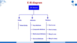
  • 33. E-R diagram ØAn Entity Relationship Diagram( ERD)- shows the relationships of a set of entities stored in a ER diagrams Øexplains the logical structure of a database. ØER based on three basic concepts: entities, attributes, and relationships.
  • 36. Company Database- Description Ø A company is organized into departments. Ø Each department has a unique name and number and is headed by a specific employee. Ø Track this employee's start date. We started leading the department. Ø Departments can have multiple locations. Ø Departments manage multiple projects with unique names, numbers, and locations. Ø Store each employee's name, social security number, address, salary, gender, and date of birth. Ø Employees are assigned to departments but work on some non-essential projects managed by the same department. Ø Track hours per Week on which employees work on all projects. Ø Also track each line manager-employee. Ø Want to track everyone's family Clerk for insurance purposes. Ø Retains name, gender, date of birth, and all family members
  • 37. E-R diagram Entities and their Attributes Ø Employee Entity : Attributes of Employee Entity are Name, Id, Address, Gender, Dob and Doj. Id is Primary Key for Employee Entity. Ø Department Entity : Attributes of Department Entity are D_no, Name and Location. D_no is Primary Key for Department Entity. Ø Project Entity : Attributes of Project Entity are P_No, Name and Location. P_No is Primary Key for Project Entity. Ø Dependent Entity : Attributes of Dependent Entity are D_name, Gender and relationship.
  • 38. E-R diagram Relationships: Employees works in Departments – Many employee works in one Department but one employee can not work in many departments. Manager controls a Department – employee works under the manager of the Department and the manager records the date of joining of employee in the department. Department has many Projects – One department has many projects but one project can not come under many departments. Employee works on project – One employee works on several projects and the number of hours worked by the employee on a single project is recorded. Employee has dependents – Each Employee has dependents. Each dependent is dependent of only one employee.
  • 40. E-R diagram -Bank Bank have Customer. Banks are identified by a name, code, address of main office. Banks have branches. Branches are identified by a branch_no., branch_name, address. Customers are identified by name, cust-id, phone number, address. Customer can have one or more accounts. Accounts are identified by account_no., acc_type, balance. Customer can avail loans. Loans are identified by loan_id, loan_type and amount. Account and loans are related to bank’s branch.
  • 41. E-R diagram -Bank Entities and their Attributes : Bank Entity : Attributes of Bank Entity are Bank Name, Code and Address. Code is Primary Key for Bank Entity. Customer Entity : Attributes of Customer Entity are Customer_id, Name, Phone Number and Address. Customer_id is Primary Key for Customer Entity. Branch Entity : Attributes of Branch Entity are Branch_id, Name and Address. Branch_id is Primary Key for Branch Entity. Account Entity : Attributes of Account Entity are Account_number, Account_Type and Balance. Account_number is Primary Key for Account Entity. Loan Entity : Attributes of Loan Entity are Loan_id, Loan_Type and Amount. Loan_id is Primary Key for Loan Entity.
  • 42. E-R diagram -Bank Relationships are : Bank has Branches => 1 : N Branch maintain Accounts => 1 : N Branch offer Loans => 1 : N Account held by Customers => M : N Loan availed by Customer => M : N
  • 44. Record Storage and Primary file organization Ø File is a collection of records. Using the primary key, we can access the records. Ø Type and frequency of access depends on the type of file organization used for a given set of records. Ø File organization is a logical relationship among various records-defines how file records are mapped onto disk blocks. Ø File organization is used to describe the way in which the records are stored in terms of blocks, and the blocks are placed on the storage medium. Ø Files of fixed length records are easier to implement than the files of variable length records.
  • 45. File organization - Objectives Ø It contains an optimal selection of records - records can be selected as fast as possible. Ø To perform insert, delete or update transaction on the records ina quick and easy way. Ø Duplicate records cannot be induced as a result of insert, update or delete. Ø With minimal cost of storage, records should be stored efficiently.
  • 46. Disk - Hardware description v The entire disk is divided into platters. v Each platter consists of concentric circles called as tracks. v These tracks are further divided into sectors which are the smallest divisions in the disk. v A cylinder is formed by combining the tracks at a given radius of a disk pack. v There exists a mechanical arm called as Read / Write head. v It is used to read from and write to the disk. v Head has to reach at a particular track and then wait for the rotation of the platter. v The rotation causes the required sector of the track to come under the head. v Each platter has 2 surfaces- top and bottom and both the surfaces are used to store the data. v Each surface has its own read / write head.
  • 47. Disk - Hardware description
  • 48. Disk - Hardware description The time taken by the disk to complete an I/O request is called as disk service time or disk access time. 1. Seek Time : Ø The time taken by the read / write head to reach the desired track is called as seek time. Ø It is the component which contributes the largest percentage of the disk service time. Ø The lower the seek time, the faster the I/O operation. 2. Rotational Latency: Ø The time taken by the desired sector to come under the read / write head is called as rotational latency. Ø It depends on the rotation speed of the spindle.
  • 49. Disk - Hardware description 3. Data Transfer Rate: Ø The amount of data that passes under the read / write head in a given amount of time is called as data transfer rate. Ø The time taken to transfer the data is called as transfer time. Ø It depends on the following factors- Ø Number of bytes to be transferred Ø Rotation speed of the disk Ø Density of the track Ø Speed of the electronics that connects the disk to the computer
  • 50. Disk - Hardware description 4. Controller Overhead: Ø The overhead imposed by the disk controller is called as controller overhead. Disk controller is a device that manages the disk. 5. Queuing Delay: Ø The time spent waiting for the disk to become free is called as queuing delay.
  • 51. Disk - Hardware description Disk access time : Disk access time = Seek time + Rotational delay + Transfer time + Controller overhead + Queuing delay
  • 52. Disk - Hardware description Disk access time : Disk access time = Seek time + Rotational delay + Transfer time + Controller overhead + Queuing delay
  • 53. Why RAID? It is a technique that combines multiple disk drives into a logical unit (RAID set) and provides protection, performance, or both. RAID RAID can be implemented by • Software RAID implementation 4 Uses host-based software to provide RAID functionality • Hardware RAID Implementation 4 Uses a specialized hardware controller installed either on a host or on an array
  • 54. RAID Techniques Three key techniques used for RAID are: Ø Striping Ø Mirroring Ø Parity
  • 55. RAID Techniques - Striping
  • 56. RAID Techniques - Mirroring
  • 58. RAID Levels • Commonly used RAID levels are: 4 RAID 0 – Striped set with no fault tolerance 4 RAID 1 – Disk mirroring 4 RAID 1 + 0 – Nested RAID 4 RAID 3 – Striped set with parallel access and dedicated parity disk 4 RAID 5 – Striped set with independent disk access and a distributed parity 4 RAID 6 – Striped set with independent disk access and dual distributed parity
  • 59. RAID Levels - RAID 0
  • 60. RAID Levels - RAID 1
  • 61. RAID Levels - RAID 1 + 0
  • 62. RAID Levels - RAID 3
  • 63. RAID Levels - RAID 5
  • 64. RAID Levels - RAID 6
  • 65. Buffering of Blocks Buffering - temporary storage of data in a buffer, or a small, fixed-sized area in memory, while it is being moved from one place to another. Two types of buffering Input buffering - temporary storage of data that is being received from an external source, such as a file on a hard drive or data being transmitted over a network. Output buffering - temporary storage of data that is being sent to an external destination, such as a printer or a file on a hard drive. In DBMS buffering is used to temporarily store data as it is being written to or read from a database. For example, when you update a record in a database, the changes may be temporarily stored in a buffer before they are written to the database.
  • 66. Buffering of Blocks -Why? ü When blocks are transferred to memory, they are held in buffers. ü If several blocks need to be transferred from the disk to main memory, several buffers can be reserved in main memory to speed up the transfer. ü While one buffer is being read/written, the CPU can process data in the other buffer which is possible because the block transfer is controlled by an independent disk I/O processor, which can transfer data blocks between main memory and the disk, independent of, and in parallel to the CPU processing data already stored in memory. ü Two ways this processing : interleaved fashion or in a parallel fashion.
  • 67. Buffering of Blocks - Benefits Improved performance − Buffering allows data to be transferred more efficiently, which can improve the overall performance of the system. Error detection and recovery − By transferring data in smaller blocks, it is easier to detect and recover from errors that may occur during the transfer process. Reduced risk of data loss − Buffering can help to prevent data loss by temporarily storing data in a buffer before it is written to a permanent storage location. Greater flexibility − Buffering allows data to be transferred asynchronously, which means that the data can be transferred at a time that is convenient for the system rather than all at once.
  • 68. How to Buffer Blocks Fixed-size block buffering Ø Buffer is divided into a fixed number of blocks,of a fixed size. Ø When data is written to the buffer, it is divided into blocks of the specified size and written to the appropriate block in the buffer. Ø Simple to implement, but it can be inefficient if the block size does not match the size of the data being written. Dynamic block buffering Ø The size of the blocks in the buffer is not fixed and the buffer is divided into a series of linked blocks, and the size of each block is determined by the amount of data that it contains. Ø Flexible than fixed-size block buffering, but it can be more complex to implement.
  • 69. How to Buffer Blocks Circular block buffering Ø Buffer is treated as a circular buffer, with data being written to the buffer and then overwriting the oldest data as the buffer becomes full. Ø Simple to implement and can be efficient, but it can lead to data loss if the data is not processed quickly enough.
  • 70. Double Buffering Ø Used in database management systems to enhance data processing and transmission. Two buffers are used, one of which is actively used for input and output activities while the second buffer gathers data for processing. Ø The buffers are switched when processing is finished which enables smooth data flow and reduces wait times.
  • 71. Double Buffering - Implementation 1. Two buffers must be created and initialised suitably in accordance with the needs of the programme. 2. Buffer manager is in charge of assigning space in the buffers for data storage after they have been set up. The buffer manager controls internal tasks and makes sure the buffers are used effectively. 3. It is possible to write to one buffer while reading from another, enabling smooth multitasking and better performance. 4. Buffers are switched when data processing is finished, ensuring a smooth transition between the old and new data sets.
  • 72. Record Blocking Types of Record Blocking 1.Fixed blocking 2. Variable-length spanned blocking 3. Variable-length unspanned blocking Records are the logical unit of a file and blocks are units of I/O with secondary storage. For I/O the records must be organized as blocks. Blocking is a process of grouping similar records into blocks that the operating system component explores exhaustively. Larger blocks reduce the I/O transfer time but requires larger I/O buffers In record blocking, the records are grouped into blocks by shared properties that are indicators of duplication.
  • 73. Record Blocking - Types 3. Variable-length unspanned blocking 1. Fixed blocking Ø Record lengths are fixed Ø Prescribed number of records stored in a block Ø Internal fragmentation is stored in a block. Ø Used for sequential files with fixed-length records
  • 74. When the block size is larger than the record size, the block will contain multiple records. Let B be the Block size and R:be the Fixed length record size in bytes. If B (size of the block) is greater that R (size of the fixed length record) then we know that we can fit B/R records per block. This is called the blocking factor (bfr). Blocking factor: bfr = ëB/Rû Unused Block Space = B – (bfr * R) bytes Blocking factor
  • 75. Record Blocking - Types 2. Variable-length spanned blocking Ø Record sizes aren’t same, Variable-length records packed into blocks with no unused space. Some records may divide into two blocks,where a pointer passes from one block to another block. So, the Pointers are used to span block unused space. Ø It is efficient in length and efficiency of storage. Ø It doesn’t limit record size, but it is more complicated to implement. So, the files are more difficult to update
  • 76. Record Blocking - Types 3. Variable-length unspanned blocking Ø Records are variable in length, but the records doesnot span between blocks. Ø In this method, the wasted area is a serious problem, because of the inability to use the remainder of a block, if the next record is larger than the remaining unused space. These blocking methods results in wasted space and limit record size to the size of the block.
  • 77. File Allocation-Methods v Define how the files are stored in the disk blocks v Aims at Efficient disk space utilization and Fast access to the file blocks. 1. Contiguous Allocation Each file occupies a contiguous set of blocks on the disk. i.e) if a file requires n blocks and is given a block b as the starting location, then the blocks assigned to the file will be: b, b+1, b+2,……b+n-1. Given the starting block address and the length of the file (in terms of blocks required), we can determine the blocks occupied by the file. The directory entry for a file with contiguous allocation contains Ø Address of starting block Ø Length of the allocated portion.
  • 78. File Allocation-Methods v Define how the files are stored in the disk blocks v Aims at Efficient disk space utilization and Fast access to the file blocks. 1. Contiguous Allocation Each file occupies a contiguous set of blocks on the disk. i.e) if a file requires n blocks and is given a block b as the starting location, then the blocks assigned to the file will be: b, b+1, b+2,……b+n-1. Given the starting block address and the length of the file (in terms of blocks required), we can determine the blocks occupied by the file. The directory entry for a file with contiguous allocation contains Ø Address of starting block Ø Length of the allocated portion.
  • 80. File Allocation-Methods 2. Linked List Allocation Each file is a linked list of disk blocks which need not be contiguous. The disk blocks can be scattered anywhere on the disk. The directory entry contains a pointer to the starting and the ending file block. Each block contains a pointer to the next block occupied by the file. The file ‘jeep’ in following image shows how the blocks are randomly distributed. The last block (25) contains -1 indicating a null pointer and does not point to any other block.
  • 81. File Allocation-Methods 3. Indexed Allocation Ø A special block known as the Index block contains the pointers to all the blocks occupied by a file. Ø Each file has its own index block. The ith entry in the index block contains the disk address of the ith file block.
  • 82. File Operations Operations on database files can be broadly classified into two categories Ø Update Operations -insertion, deletion, or update Ø Retrieval Operations -locate certain records so their field values can be examined and processed. Ø Record-at –a time operation or Set-at-a-time operations File Processing happens as: Ø Open − A file can be opened in one of the two modes, read mode or write mode Ø Locate − Every file has a file pointer, which tells the current position where the data is to be read or written. Ø Read − By default, when files are opened in read mode, the file pointer points to the beginning of the file. Ø Write − User can select to open a file in write mode, which enables them to edit its contents. It can be deletion, insertion, or modification. Ø Close − removes all the locks ,saves the data to the secondary storage media and Ø releases all the buffers and file handlers associated with the file.
  • 83. File Organisations A file organisation refers to the the way records and blocks are placed on the storage medium and linked. Some types of File Organizations are : 1. Sequential File Organization : File is stored one after another in a sequential manner. 1. Pile File Method - store the records in a sequence i.e. one after the other in the order in which they are inserted into the tables-new one at end 2. Sorted File Method - new record is always inserted in a sorted (ascending or descending) manner. The sorting of records may be based on any primary key or any other key.
  • 84. File Organisations 2. Heap File Organization Ø records are inserted at the end of the file, into the data blocks. Ø No Sorting or Ordering is required in this method. Ø If a data block is full, the new record is stored in some other block, Here the other data block need not be the very next data block, but it can be any block in the memory. Ø It is the responsibility of DBMS to store and manage the new records.
  • 85. File Organisations 3. Hash File Organization : Ø Also called a direct file organisation. Ø For storing the records a hash function is calculated on some fields of the record, which provides the address of the block to store the record. Any type of mathematical function can be used as a hash function Ø Hashing uses a hash function, h, that is applied to the hash field value of a record and gives the address of the disk block in which the record is stored.
  • 86. File Organisations 3. Hash File Organization : Ø Also called a direct file organisation. Ø For storing the records a hash function is calculated on some fields of the record, which provides the address of the block to store the record. Any type of mathematical function can be used as a hash function Ø Hashing uses a hash function, h, that is applied to the hash field value of a record and gives the address of the disk block in which the record is stored.
  • 87. Internal Hashing Ø For internal files, hashing is typically implemented as a hash table through the use of an array of records. Ø Suppose that the array index range is from 0 to M – 1, then we have M slots whose addresses correspond to the array indexes. Ø We choose a hash function that transforms the hash field value into an integer between 0 and M − 1. Ø One common hash function is the h(K) = K mod M function, which returns the remainder of an integer hash field value K after division by M; this value is then used for the record address. Ø Noninteger hash field values can be transformed into integers before the mod function is applied.
  • 89. Internal Hashing Ø Folding involves applying an arithmetic function such as addition or logical function such as exclusive or (Xor) to different portions of the hash field value to calculate the hash address. Ø Another technique involves picking some digits of the hash field value (ie. Third, fifth, eighth digits) to form the hash address. Problem: Ø hashing functions is that they don’t guarantee that distinct values will hash to distinct addresses- Many values can hash to the same address Ø This is because the hash field space is much larger than the address space .
  • 90. Collision Resolution Mechanisms Open Addressing/Linear Probing : Ø if the hash address is occupied, the program checks the next positions in order until an empty address is found. Chaining : Ø Overflow locations are used, by extending the array with overflow positions. Ø Each record location has a pointer field, and if the hash address is occupied, the collision is resolved by placing the new record in an unused overflow location, and setting the pointer of the occupied hash address location to the address of the overflow location. Ø A linked list of the overflow records for each hash address is maintained. Multiple hashing : Ø If the first hash function results in a collision, a second hash function is applied. If there is a collision after the second hash function, either a third hash function is applied, or open addressing is used.
  • 91. External Hashing Ø Hashing for disk files is called external hashing. Ø The target address space is made up of buckets (blocks).A bucket can be either one disk block, or multiple contiguous blocks. Ø Each bucket holds multiple records. Ø The hashing function maps a key into a relative bucket number, rather than assign an absolute block address to the bucket. Ø A table maintained in the file header converts the bucket number into the corresponding block address Ø the collision problem is less severe, because many records can hash to the same bucket. and if a bucket becomes full and new records hashing to a full bucket, collision resolving mechanisms again must be used. Ø every bucket maintains a pointer to a linked list of overflow records for that bucket.
  • 92. External Hashing Ø This hashing scheme is called static hashing because a fixed number of buckets, M, is allocated for the address space. If m is the maximum number of records that can fit into a bucket, the total capacity allocated for all buckets is (M * m). If there are significantly fewer than (M * m) records, then there is a lot of unused record space.And if there are more than (M*m) records numerous collisions will result, and performance will be affected because of the long lists of overflow records. Ø Searching for a record when using external hashing is expensive if the search field is not the hash field. Ø Record deletion can be implemented by removing the record from its bucket. If the bucket has an overflow chain, the overflow records can be moved into the bucket to replace the deleted record.
  • 94. External Hashing -Dynamic File Expansion Ø In static hashing is that address space is fixedand indynamic file organizations based on hashing allow the number of buckets to vary dynamically with only localised reorganization.
  • 95. External Hashing-Dynamic File Expansion Extendible Hashing Ø based on binary representation of a number. Ø Apply a hashing function to a non negative integer, and represent the result as a binary number- a string of bits -which is called the hash value of a record. Ø Records are distributed among buckets based on the values of the leading bits in their hash values. Ø a directory of 2d bucket addresses in maintained, d is the global depth of the directory. Ø The integer value corresponding to the first d bits of a hash value is used as an index to the array to determine a directory entry, and the address in the directory entry determines the bucket in which the corresponding records are stored.
  • 96. External Hashing - Dynamic File Expansion Extendible Hashing Ø A local depth, d1 stored with each bucket specifies the number of bits on which the bucket contents are based. Ø The value d can be increased or decreased by one at a time, doubling or halving the number of entries in the directory.
  • 97. External Hashing - Dynamic File Expansion Linear Hashing Ø allows a hash file to expand and shrink its number of buckets dynamically without needing a directory. Ø The file starts with M buckets, numbered 0 to M-1, and uses the initial hash function h(K)= K mod M. Overflow because of collisions is needed, and can be handled using an overflow chain for each bucket. Ø When a collision leads to an overflow record in ANY file bucket, the first bucket is split into two buckets, the original bucket 0, and a new bucket M at the end of the file. The records in bucket 0 are distributed between the two buckets based on a different hashing function, hi+1(K) = K mod M.
  • 98. File Organisations 2. Heap File Organization records are inserted at the end of the file, into the data blocks. No Sorting or Ordering is required in this method. If a data block is full, the new record is stored in some other block, Here the other data block need not be the very next data block, but it can be any block in the memory. It is the responsibility of DBMS to store and manage the new records.