


Unit 3 Network Layer PPT
- 1. KARPAGAM INSTITUTE OF TECHNOLOGY DEPARTMENT OF COMPUTER SCIENCE AND ENGINEERING Course Code with Name :CS8591/Computer Networks Staff Name / Designation : Mrs.C.Kalpana / AP Department : CSE Year/Semester : III/V 1 Karpagam Institute of Technology 4/5/2022
- 2. UNIT III NETWORK LAYER 4/5/2022 Karpagam Institute of Technology 2 Network Layer Services – Packet switching – Performance – IPV4 Addresses – Forwarding of IP Packets - Network Layer Protocols: IP, ICMP v4 – Unicast Routing Algorithms – Protocols – Multicasting Basics – IPV6 Addressing – IPV6 Protocol.
- 3. Network Layer The Network Layer is the third layer of the OSI model. It handles the service requests from the transport layer and further forwards the service request to the data link layer. The network layer translates the logical addresses into physical addresses It determines the route from the source to the destination and also manages the traffic problems such as switching, routing and controls the congestion of data packets. The main role of the network layer is to move the packets from sending host to the receiving host. 4/5/2022 Karpagam Institute of Technology 3
- 4. Functions of Network Layer Routing: When a packet reaches the router's input link, the router will move the packets to the router's output link. For example, a packet from S1 to R1 must be forwarded to the next router on the path to S2. Logical Addressing: The data link layer implements the physical addressing and network layer implements the logical addressing. Logical addressing is also used to distinguish between source and destination system. The network layer adds a header to the packet which includes the logical addresses of both the sender and the receiver. 4/5/2022 Karpagam Institute of Technology 4
- 5. Functions of Network Layer Internetworking: This is the main role of the network layer that it provides the logical connection between different types of networks. Fragmentation: The fragmentation is a process of breaking the packets into the smallest individual data units that travel through different networks. 4/5/2022 Karpagam Institute of Technology 5
- 6. 4/5/2022 Karpagam Institute of Technology 6
- 7. Features Main responsibility of Network layer is to carry the data packets from the source to the destination without changing or using it. If the packets are too large for delivery, they are fragmented i.e., broken down into smaller packets. It decides the root to be taken by the packets to travel from the source to the destination among the multiple roots available in a network (also called as routing). The source and destination addresses are added to the data packets inside the network layer. 4/5/2022 Karpagam Institute of Technology 7
- 8. Network Layer Services Guaranteed delivery: This layer provides the service which guarantees that the packet will arrive at its destination. Guaranteed delivery with bounded delay: This service guarantees that the packet will be delivered within a specified host-to-host delay bound. In-Order packets: This service ensures that the packet arrives at the destination in the order in which they are sent. 4/5/2022 Karpagam Institute of Technology 8
- 9. Network Layer Services Guaranteed max jitter: This service ensures that the amount of time taken between two successive transmissions at the sender is equal to the time between their receipt at the destination. Security services: The network layer provides security by using a session key between the source and destination host. The network layer in the source host encrypts the payloads of datagrams being sent to the destination host. The network layer in the destination host would then decrypt the payload. In such a way, the network layer maintains the data integrity and source authentication services. 4/5/2022 Karpagam Institute of Technology 9
- 10. Other services in Network Layer Error Control: Although it can be implemented in the network layer, but it is usually not preferred because the data packet in a network layer maybe fragmented at each router, which makes error checking inefficient in the network layer. Congestion Control: Congestion occurs when the number of datagrams sent by source is beyond the capacity of network or routers. This is another issue in the network layer protocol. If congestion continues, sometimes a situation may arrive where the system collapses and no datagrams are delivered. Although congestion control is indirectly implemented in network layer, but still there is a lack of congestion control in the network layer. 4/5/2022 Karpagam Institute of Technology 10
- 11. Other services in Network Layer Flow Control: It regulates the amount of data a source can send without overloading the receiver. If the source produces a data at a very faster rate than the receiver can consume it, the receiver will be overloaded with data. To control the flow of data, the receiver should send a feedback to the sender to inform the latter that it is overloaded with data. There is a lack of flow control in the design of the network layer. It does not directly provide any flow control. The datagrams are sent by the sender when they are ready, without any attention to the readiness of the receiver. 4/5/2022 Karpagam Institute of Technology 11
- 12. Advantages of Network Layer services Packetization service in network layer provides an ease of transportation of the data packets. Packetization also eliminates single points of failure in data communication systems. Routers present in the network layer reduce network traffic by creating collision and broadcast domains. With the help of Forwarding, data packets are transferred from one place to another in the network. 4/5/2022 Karpagam Institute of Technology 12
- 13. Disadvantages of Network Layer services There is a lack of flow control in the design of the network layer. Congestion occurs sometimes due to the presence of too many datagrams in a network which are beyond the capacity of network or the routers. Due to this, some routers may drop some of the datagrams and some important piece of information maybe lost. Although indirectly error control is present in network layer, but there is a lack of proper error control mechanisms as due to presence of fragmented data packets, error control becomes difficult to implement. 4/5/2022 Karpagam Institute of Technology 13
- 14. Packet switching Packet switching is a method of transferring the data to a network in form of packets. In order to transfer the file fast and efficient manner over the network and minimize the transmission latency, the data is broken into small pieces of variable length, called Packet. At the destination, all these small-parts (packets) has to be reassembled, belonging to the same file. A packet composes of payload and various control information. No pre-setup or reservation of resources is needed. 4/5/2022 Karpagam Institute of Technology 14
- 15. Packet switching Packet Switching uses Store and Forward technique while switching the packets; while forwarding the packet each hop first store that packet then forward. This technique is very beneficial because packets may get discarded at any hop due to some reason. Packet-Switched networks were designed to overcome the weaknesses of Circuit-Switched networks since circuit-switched networks were not very effective for small messages. 4/5/2022 Karpagam Institute of Technology 15
- 16. Advantages of Packet Switching More efficient in terms of bandwidth, since the concept of reserving circuit is not there. Minimal transmission latency. More reliable as destination can detect the missing packet. More fault tolerant because packets may follow different path in case any link is down, Unlike Circuit Switching. Cost effective and comparatively cheaper to implement. 4/5/2022 Karpagam Institute of Technology 16
- 17. Disadvantages of Packet Switching Packet Switching don’t give packets in order, whereas Circuit Switching provides ordered delivery of packets because all the packets follow the same path. Since the packets are unordered, we need to provide sequence numbers to each packet. Complexity is more at each node because of the facility to follow multiple path. Transmission delay is more because of rerouting. Packet Switching is beneficial only for small messages, but for bursty data (large messages) Circuit Switching is better. 4/5/2022 Karpagam Institute of Technology 17
- 18. Modes in packet switching Connection oriented packet switching Connection less packet switching 4/5/2022 Karpagam Institute of Technology 18
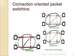
- 19. Connection oriented packet switching Before starting the transmission, it establishes a logical path or virtual connection using signalling protocol, between sender and receiver and all packets belongs to this flow will follow this predefined route. Virtual Circuit ID is provided by switches/routers to uniquely identify this virtual connection. Data is divided into small units and all these small units are appended with help of sequence number. Overall, three phases takes place here- Setup, data transfer and tear down phase. 4/5/2022 Karpagam Institute of Technology 19
- 20. Connection oriented packet switching 4/5/2022 Karpagam Institute of Technology 20
- 21. Connection oriented packet switching 4/5/2022 Karpagam Institute of Technology 21 All address information is only transferred during setup phase. Once the route to destination is discovered, entry is added to switching table of each intermediate node. During data transfer, packet header (local header) may contain information such as length, timestamp, sequence number etc. Connection-oriented switching is very useful in switched WAN. Some popular protocols which use Virtual Circuit Switching approach are X.25, Frame-Relay, ATM and MPLS(Multi- Protocol Label Switching).
- 22. Connectionless packet switching In Connectionless Packet Switching each packet contains all necessary addressing information such as source address, destination address and port numbers etc. In Datagram Packet Switching, each packet is treated independently. Packets belonging to one flow may take different routes because routing decisions are made dynamically, so the packets arrived at destination might be out of order. It has no connection setup and teardown phase, like Virtual Circuits. Packet delivery is not guaranteed in connectionless packet switching, so the reliable delivery must be provided by end systems using additional protocols. 4/5/2022 Karpagam Institute of Technology 22
- 23. Connectionless packet switching 4/5/2022 Karpagam Institute of Technology 23
- 24. Delays in packet switching Transmission Delay Propagation Delay Queuing Delay Processing Delay 4/5/2022 Karpagam Institute of Technology 24
- 25. Transmission Delay Time taken to put a packet onto link. In other words, it is simply time required to put data bits on the wire/communication medium. It depends on length of packet and bandwidth of network. Transmission Delay = Data size / bandwidth = (L/B) second 4/5/2022 Karpagam Institute of Technology 25
- 26. Propagation Delay Time taken by the first bit to travel from sender to receiver end of the link. In other words, it is simply the time required for bits to reach the destination from the start point. Factors on which Propagation delay depends are Distance and propagation speed. Propagation delay = distance/transmission speed = d/s 4/5/2022 Karpagam Institute of Technology 26
- 27. Queuing Delay Queuing delay is the time a job waits in a queue until it can be executed. It depends on congestion. It is the time difference between when the packet arrived Destination and when the packet data was processed or executed. It may be caused by mainly three reasons i.e. originating switches, intermediate switches or call receiver servicing switches. Average Queuing delay = (N-1)L/(2*R) where N = no. of packets L=size of packet R=bandwidth 4/5/2022 Karpagam Institute of Technology 27
- 28. Processing Delay Processing delay is the time it takes routers to process the packet header. Processing of packets helps in detecting bit-level errors that occur during transmission of a packet to the destination. Processing delays in high-speed routers are typically on the order of microseconds or less. In simple words, it is just the time taken to process packets. 4/5/2022 Karpagam Institute of Technology 28
- 29. Processing Delay Total time or End-to-End time = Transmission delay + Propagation delay+ Queuing delay + Processing delay For M hops and N packets – Total delay = M*(Transmission delay + propagation delay)+ (M-1)*(Processing delay + Queuing delay) + (N-1)*(Transmission delay) For N connecting link in the circuit – Transmission delay = N*L/R Propagation delay = N*(d/s) 4/5/2022 Karpagam Institute of Technology 29
- 30. Problem How much time will it take to send a packet of size L bits from A to B in given setup if Bandwidth is R bps, propagation speed is t meter/sec and distance b/w any two points is d meters (ignore processing and queuing delay) ? A---R1---R2---B Ans: N = no. of links = no. of hops = no. of routers +1 = 3 File size = L bits Bandwidth = R bps Propagation speed = t meter/sec Distance = d meters Transmission delay = (N*L)/R = (3*L)/R sec Propagation delay = N*(d/t) = (3*d)/t sec Total time = 3*(L/R + d/t) sec 4/5/2022 Karpagam Institute of Technology 30
- 31. IPV4 address An IP address (internet protocol address) is a numerical representation that uniquely identifies a specific interface on the network. Addresses in IPv4 are 32-bits long. This allows for a maximum of 4,294,967,296 (232) unique addresses. Addresses in IPv6 are 128-bits, which allows for 3.4 x 1038 (2128) unique addresses. 4/5/2022 Karpagam Institute of Technology 31
- 32. IPV4 Address IP addresses are binary numbers but are typically expressed in decimal form (IPv4) or hexadecimal form (IPv6) to make reading and using them easier for humans. IP stands for Internet Protocol and describes a set of standards and requirements for creating and transmitting data packets, or datagrams, across networks. The Internet Protocol (IP) is part of the Internet layer of the Internet protocol suite. In the OSI model, IP would be considered part of the network layer. IP is traditionally used in conjunction with a higher-level protocol, most notably TCP. The IP standard is governed by RFC 791. 4/5/2022 Karpagam Institute of Technology 32
- 33. 4/5/2022 Karpagam Institute of Technology 33
- 34. IPV4 Address IPv4 addresses are actually 32-bit binary numbers, consisting of the two sub addresses (identifiers) mentioned above which, respectively, identify the network and the host to the network, with an imaginary boundary separating the two. An IP address is, as such, generally shown as 4 octets of numbers from 0-255 represented in decimal form instead of binary form. An IPv4 address is typically expressed in dotted- decimal notation, with every eight bits (octet) represented by a number from one to 255, each separated by a dot. An example IPv4 address would look like this: 192.168.17.12 4/5/2022 Karpagam Institute of Technology 34
- 36. Fragmentation and Reassembly Fragmentation and reassembly is a method for transmission of messages larger than networks Maximum Transmission Unit (MTU). Messages are fragmented into small pieces by the sender and reassembled by the receiver. 4/5/2022 Karpagam Institute of Technology 36
- 37. Fragmentation and Reassembly 4/5/2022 Karpagam Institute of Technology 37
- 38. Fragmentation and Reassembly 4/5/2022 Karpagam Institute of Technology 38
- 39. Global Address The term IP address is used to mean a logical address in the network layer and is used in the Source address and Destination address field of the IP packets. 4/5/2022 Karpagam Institute of Technology 39
- 40. Logical Address Logical address are necessary for universal communications to identify each host in the internet for delivery of a packet from host to host. All IPv4 addresses are 32 bits long ( equivalently 4 bytes). Within an IP address it encodes its network number and host number. The physical (network) addresses will change from hop to hop, but the logical addresses remains the same. 4/5/2022 Karpagam Institute of Technology 40
- 41. Network id and Host id Network ID is the portion of an IP address that identifies the TCP/IP network on which a host resides. The network ID portion of an IP address uniquely identifies the host’s network on an internetwork, while the host ID portion of the IP address identifies the host within its network. Together, the host ID and network ID, which make up the entire IP address of a host, uniquely identify the host on a TCP/IP internetwork. 4/5/2022 Karpagam Institute of Technology 41
- 42. Address Space An address space is the total number of addresses used by the protocol. For an N bits address, 2N bits address space can be used, because each bit can have two different values (0 or 1). 4/5/2022 Karpagam Institute of Technology 42
- 43. Notations Two types of notations in IPv4. 1. Binary Notation 2. Dotted- Decimal Notation 4/5/2022 Karpagam Institute of Technology 43
- 44. Binary Notation The binary notation in IPv4 is a 32 bit address or 4 bytes addres. Ex; 01000000 00100000 00010000 00000111 4/5/2022 Karpagam Institute of Technology 44
- 45. Dotted- Decimal Notation To make 32 bit form shorter and easier to read, Internet addresses are usually written in Decimal form with decimal points separating the bytes called as Dotted decimal notation. Each number varies from 0 to 255. Example: 01000000 00100000 00010000 00000111 64 32 16 7 4/5/2022 Karpagam Institute of Technology 45
- 46. Classful Addressing IPv4 addresses were divided into 5 categories. ◦ Class A ◦ Class B ◦ Class C ◦ Class D ◦ Class E This allocation has come to be called classful addressing 4/5/2022 Karpagam Institute of Technology 46
- 47. Classful Addressing IPv4 address of 4 bytes defines 3 fields. Class Type Network ID(Netid) HostID 4/5/2022 Karpagam Institute of Technology 47
- 48. Class A Class A addresses were designed for large organizations with a large number of attached hosts or routers. In a Class A network, the first eight bits, or the first dotted decimal, is the network part of the address, with the remaining part of the address being the host part of the address. There are 128 possible Class A networks. 0.0.0.0 to 127.0.0.0 However, any address that begins with 127. is considered a loopback address. 4/5/2022 Karpagam Institute of Technology 48
- 49. Class B Class B addresses were designed for midsize organizations with tens of thousands of attached hosts or routers. In a Class B network, 2 bytes for class type and netid and 2 bytes for hosted. All Class B networks have their first bit set to 1 and the second bit set to 0. In dotted decimal notation, that makes 128.0.0.0 to 191.255.0.0 as Class B networks. There are 16,384 possible Class B networks. Example for a Class B IP address: 135.168.24.14 4/5/2022 Karpagam Institute of Technology 49
- 50. Class C Class C addresses were designed for small organizations with a small number of attached hosts or routers. It uses 3 bytes for class type and netid and 1 byte for hostid. In a Class C network, the first two bits are set to 1, and the third bit is set to 0. That makes the first 24 bits of the address the network address and the remainder as the host address. Class C network addresses range from 192.0.0.0 to 223.255.255.0. There are over 2 million possible Class C networks. 192.168.178.1 4/5/2022 Karpagam Institute of Technology 50
- 51. Class D Class D addresses are used for multicasting applications. Class D addresses have their first three bits set to “1” and their fourth bit set to “0”. Class D addresses are 32-bit network addresses, meaning that all the values within the range of 224.0.0.0 – 239.255.255.255 are used to uniquely identify multicast groups. There are no host addresses within the Class D address space, since all the hosts within a group share the group’s IP address for receiver purposes. 227.16.6.176 4/5/2022 Karpagam Institute of Technology 51
- 52. Class E Class E addresses are reserved for future use, in which addresses beginning with 1111. Class E networks are defined by having the first four network address bits as 1. That encompasses addresses from 240.0.0.0 to 255.255.255.255. While this class is reserved, its usage was never defined. As a result, most network implementations discard these addresses as illegal or undefined. 243.164.89.28 4/5/2022 Karpagam Institute of Technology 52
- 53. Classful Addressing 4/5/2022 Karpagam Institute of Technology 53
- 54. Classful Addressing 4/5/2022 Karpagam Institute of Technology 54
- 55. Classful Addressing 4/5/2022 Karpagam Institute of Technology 55
- 56. 4/5/2022 Karpagam Institute of Technology 56
- 57. 4/5/2022 Karpagam Institute of Technology 57
- 58. 4/5/2022 Karpagam Institute of Technology 58 Solution We replace each group of 8 bits with its equivalent decimal number (see Appendix B) and add dots for separation. Change the following IPv4 addresses from binary notation to dotted- decimal notation.
- 59. 4/5/2022 Karpagam Institute of Technology 59
- 60. 4/5/2022 Karpagam Institute of Technology 60
- 61. 4/5/2022 Karpagam Institute of Technology 61
- 62. Disadvantages of Classful Addressing If we consider class A, the number of addresses in each block is more than enough for almost any organization. So, it results in wastage of addresses. Same is the case with class B, probably an organization receiving block from class B would not require that much of addresses. So, it also results in wastage of addresses. A block in class C may be too small to fulfil the addresses requirement of an organization. Each address in class D defines a group of hosts. Hosts need to multicast the address. So, the addresses are wasted here too. Addresses of class E are reserved for the future purpose which is also wastage of addresses. The main issue here is; we are not assigning addresses according to user requirements. We directly assign a block of a fixed size which has a fixed number of addresses which leads to wastage of address. 4/5/2022 Karpagam Institute of Technology 62
- 63. Subnetting and Supernetting To overcome the flaws of classful addressing, these two solutions were introduced to compensate for the wastage of addresses. Let us discuss them one by one. 4/5/2022 Karpagam Institute of Technology 63
- 64. Subnetting As class blocks of A & B are too large for any organization. So, they can divide their large network in the smaller subnetwork and share them with other organizations. This whole concept is subnetting. Supernetting As the blocks in class A and B were almost consumed so, new organizations consider class C. But, the block of class C is too small then the requirement of the organization. In this case, the solution which came out is supernetting which grants to join the blocks of class C to form a larger block which satisfies the address requirement of the organization. 4/5/2022 Karpagam Institute of Technology 64
- 65. Subnetting A subnet, or subnetwork, is a segmented piece of a larger network. More specifically, subnets are a logical partition of an IP network into multiple, smaller network segments. Organizations will use a subnet to subdivide large networks into smaller, more efficient subnetworks. 4/5/2022 Karpagam Institute of Technology 65
- 66. Private Address Within the address space, certain networks are reserved for private networks. Packets from these networks are not routed across the public internet. This provides a way for private networks to use internal IP addresses without interfering with other networks. The private networks are 10.0.0.1 - 10.255.255.255 172.16.0.0 - 172.32.255.255 192.168.0.0 - 192.168.255.255 4/5/2022 Karpagam Institute of Technology 66
- 67. 4/5/2022 Karpagam Institute of Technology 67
- 68. Subnetting and Super netting Subnetting is the procedure to divide the network into sub- networks or small networks. Super netting is the procedure of combine the small networks into larger space. In subnetting, Network addresses’s bits are increased. on the other hand, in subnetting, Host addresses’s bits are increased. Subnetting is implemented via Variable-length subnet masking, While supernetting is implemented via Classless interdomain routing. 4/5/2022 Karpagam Institute of Technology 68
- 69. 4/5/2022 Karpagam Institute of Technology 69
- 70. 4/5/2022 Karpagam Institute of Technology 70
- 71. Subnetting When a bigger network is divided into smaller networks, in order to maintain security, then that is known as Subnetting. so, maintenance is easier for smaller networks. 4/5/2022 Karpagam Institute of Technology 71
- 72. What is the subnetwork address if the destination address is 200.45.34.56 and the subnet mask is 255.255.240.0 ? Solution: Convert the given destination address into binary format. 200.45.34.56 = 11001000 00101101 00100010 00111000 Convert the given subnet mask into binary format. 255.255.240.0 = 11111111 11111111 11110000 00000000 Do the AND operation using destination address and subnet mask address. 200.45.34.56 = 11001000 00101101 00100010 00111000 255.255.240.0 = 11111111 11111111 11110000 00000000 11001000 00101101 00100000 00000000 subnetwork address is 200.45.32.0 4/5/2022 Karpagam Institute of Technology 72
- 73. Find the subnetwork address for the following: S.No IP address Mask A 140.11.36.22 255.255.255.0 Solution: IP address 140.11.36.22 Mask 255.255.255.0 140.11.36.0 4/5/2022 Karpagam Institute of Technology 73
- 74. CLASSLESS ADDRESSING In classless addressing, variable-length blocks are used that belong to no classes. We can have a block of 1 address, 2 addresses, 4 addresses, 128 addresses, and so on. In classless addressing, the whole address space is divided into variable length blocks. The prefix in an address defines the block (network); the suffix defines the node (device). The number of addresses in a block needs to be a power of 2. An organization can be granted one block of addresses. 4/5/2022 Karpagam Institute of Technology 74
- 75. CLASSLESS ADDRESSING 4/5/2022 Karpagam Institute of Technology 75 • The prefix length in classless addressing is variable. • We can have a prefix length that ranges from 0 to 32. • The size of the network is inversely proportional to the length of the prefix. • A small prefix means a larger network; a large prefix means a smaller network. • The idea of classless addressing can be easily applied to classful addressing. • An address in class A can be thought of as a classless address in which the prefix length is 8. • An address in class B can be thought of as a classless address in which the prefix is 16, and so on. In other words, classful addressing is a special case of classless addressing.
- 76. Notation used in Classless Addressing The notation used in classless addressing is informally referred to as slash notation and formally as classless interdomain routing or CIDR. For example , 192.168.100.14 /24 represents the IP address 192.168.100.14 and, its subnet mask 255.255.255.0, which has 24 leading 1-bits. 4/5/2022 Karpagam Institute of Technology 76
- 77. Address Aggregation One of the advantages of the CIDR strategy is address aggregation (sometimes called address summarization or route summarization). When blocks of addresses are combined to create a larger block, routing can be done based on the prefix of the larger block. ICANN assigns a large block of addresses to an ISP. Each ISP in turn divides its assigned block into smaller subblocks and grants the subblocks to its customers. 4/5/2022 Karpagam Institute of Technology 77
- 78. Special Addresses in IPv4 There are five special addresses that are used for special purposes: this-host address, limited-broadcast address, loopback address, private addresses, and multicast addresses. 4/5/2022 Karpagam Institute of Technology 78
- 79. This-host Address The only address in the block 0.0.0.0/32 is called the this-host address. It is used whenever a host needs to send an IP datagram but it does not know its own address to use as the source address. 4/5/2022 Karpagam Institute of Technology 79
- 80. Limited-broadcast Address The only address in the block 255.255.255.255/32 is called the limitedbroadcast address. It is used whenever a router or a host needs to send a datagram to all devices in a network. The routers in the network, however, block the packet having this address as the destination;the packet cannot travel outside the network. 4/5/2022 Karpagam Institute of Technology 80
- 81. Loopback Address The block 127.0.0.0/8 is called the loopback address. A packet with one of the addresses in this block as the destination address never leaves the host; it will remain in the host. Private Addresses Four blocks are assigned as private addresses: 10.0.0.0/8, 172.16.0.0/12, 192.168.0.0/16, and 169.254.0.0/16. Multicast Addresses The block 224.0.0.0/4 is reserved for multicast addresses. 4/5/2022 Karpagam Institute of Technology 81
- 82. DHCP – DYNAMIC HOST CONFIGURATION PROTOCOL The dynamic host configuration protocol is used to simplify the installation and maintenance of networked computers. DHCP is derived from an earlier protocol called BOOTP. Ethernet addresses are configured into network by manufacturer and they are unique. IP addresses must be unique on a given internetwork but also must reflect the structure of the internetwork. The main goal of DHCP is to minimize the amount of manual configuration required for a host. 4/5/2022 Karpagam Institute of Technology 82
- 83. If a new computer is connected to a network, DHCP can provide it with all the necessary information for full system integration into the network. DHCP is based on a client/server model. DHCP clients send a request to a DHCP server to which the server responds with an IP address DHCP server is responsible for providing configuration information to hosts. There is at least one DHCP server for an administrative domain. The DHCP server can function just as a centralized repository for host configuration information. The DHCP server maintains a pool of available addresses that it hands out to hosts on demand. 4/5/2022 Karpagam Institute of Technology 83
- 84. DHCP – DYNAMIC HOST CONFIGURATION PROTOCOL 4/5/2022 Karpagam Institute of Technology 84
- 85. DHCP – DYNAMIC HOST CONFIGURATION PROTOCOL A newly booted or attached host sends a DHCPDISCOVER message to a special IP address (255.255.255.255., which is an IP broadcast address. This means it will be received by all hosts and routers on that network. DHCP uses the concept of a relay agent. There is at least one relay agent on each network. DHCP relay agent is configured with the IP address of the DHCP server. When a relay agent receives a DHCPDISCOVER message, it unicasts it to the DHCP server and awaits the response, which it will then send back to the requesting client. 4/5/2022 Karpagam Institute of Technology 85
- 86. DHCP – DYNAMIC HOST CONFIGURATION PROTOCOL 4/5/2022 Karpagam Institute of Technology 86
- 87. DHCP Message Format 4/5/2022 Karpagam Institute of Technology 87
- 88. NETWORK ADDRESS TRANSLATION (NAT) A technology that can provide the mapping between the private and universal (external)addresses, and at the same time support virtual private networks is called as Network Address Translation (NAT). The technology allows a site to use a set of private addresses for internal communication and a set of global Internet addresses (at least one) for communication with the rest of the world. The site must have only one connection to the global Internet through a NAT capable router that runs NAT software. 4/5/2022 Karpagam Institute of Technology 88
- 89. NETWORK ADDRESS TRANSLATION (NAT) 4/5/2022 Karpagam Institute of Technology 89
- 90. Types of NAT Two types of NAT exists . (a) One-to-one translation of IP addresses (b) One-to-many translation of IP addresses 4/5/2022 Karpagam Institute of Technology 90
- 91. Address Translation All of the outgoing packets go through the NAT router, which replaces the source address in the packet with the global NAT address. All incoming packets also pass through the NAT router, which replaces the destination address in the packet (the NAT router global address) with the appropriate private address. Translation Table There may be tens or hundreds of private IP addresses, each belonging to one specific host. The problem arises when we want to translate the source address to an external 4/5/2022 Karpagam Institute of Technology 91
- 92. Network Layer Protocols: IP The IP (Internet Protocol) is a protocol that uses datagrams to communicate over a packet-switched network. The IP protocol operates at the network layer protocol of the OSI reference model and is a part of a suite of protocols known as TCP/IP. The IP network service transmits datagrams between intermediate nodes using IP routers. 4/5/2022 Karpagam Institute of Technology 92
- 93. Network Layer Protocols: IP The routers themselves are simple, since no information is stored concerning the datagrams which are forwarded on a link. The most complex part of an IP router is concerned with determining the optimum link to use to reach each destination in a network. This process is known as "routing". Although this process is computationally intensive, it is only performed at periodic intervals. 4/5/2022 Karpagam Institute of Technology 93
- 94. ICMP-Internet Control Message Protocol Since IP does not have a inbuilt mechanism for sending error and control messages. It depends on Internet Control Message Protocol(ICMP) to provide an error control. It is used for reporting errors and management queries. It is a supporting protocol and used by networks devices like routers for sending the error messages and operations information. e.g. the requested service is not available or that a host or router could not be reached. 4/5/2022 Karpagam Institute of Technology 94
- 95. ICMP The Internet Control Message Protocol (ICMP) is a network layer protocol used by network devices to diagnose network communication issues. ICMP is mainly used to determine whether or not data is reaching its intended destination in a timely manner. Commonly, the ICMP protocol is used on network devices, such as routers. ICMP is crucial for error reporting and testing, but it can also be used in distributed denial-of-service (DDoS) attacks. 4/5/2022 Karpagam Institute of Technology 95
- 96. What is ICMP used for? The primary purpose of ICMP is for error reporting. When two devices connect over the Internet, the ICMP generates errors to share with the sending device in the event that any of the data did not get to its intended destination. For example, if a packet of data is too large for a router, the router will drop the packet and send an ICMP message back to the original source for the data. 4/5/2022 Karpagam Institute of Technology 96
- 97. A secondary use of ICMP protocol is to perform network diagnostics; the commonly used terminal utilities traceroute and ping both operate using ICMP. The traceroute utility is used to display the routing path between two Internet devices. The routing path is the actual physical path of connected routers that a request must pass through before it reaches its destination. The journey between one router and another is known as a ‘hop,’ and a traceroute also reports the time required for each hop along the way. This can be useful for determining sources of network delay. 4/5/2022 Karpagam Institute of Technology 97
- 98. ICMP MESSAGE TYPES ICMP messages are divided into two broad categories: error-reporting messages and query messages. The error-reporting messages report problems that a router or a host (destination) may encounter when it processes an IP packet. The query messages help a host or a network manager get specific information from a router or another host. 4/5/2022 Karpagam Institute of Technology 98
- 99. 4/5/2022 Karpagam Institute of Technology 99
- 100. ICMP Error – Reporting Messages 4/5/2022 Karpagam Institute of Technology 100
- 101. Destination Unreachable―When a router cannot route a datagram, the datagram is discarded and sends a destination unreachable message to source host. Source Quench―When a router or host discards a datagram due to congestion, it sends a source-quench message to the source host. This message acts as flow control. Time Exceeded―Router discards a datagram when TTL field becomes 0 and a time exceeded message is sent to the source host. Parameter Problem―If a router discovers ambiguous or missing value in any field of the datagram, it discards the datagram and sends parameter problem message to source. Redirection―Redirect messages are sent by the default router to inform the source host to update its forwarding table when the packet is routed on a wrong path. 4/5/2022 Karpagam Institute of Technology 101
- 102. Source quench message Source quench message is request to decrease traffic rate for messages sending to the host(destination). Or we can say, when receiving host detects that rate of sending packets (traffic rate) to it is too fast it sends the source quench message to the source to slow the pace down so that no packet can be lost. 4/5/2022 Karpagam Institute of Technology 102
- 103. ICMP will take source IP from the discarded packet and informs to source by sending source quench message. Then source will reduce the speed of transmission so that router will free for congestion. When the congestion router is far away from the source the ICMP will send hop by hop source quench message so that every router will reduce the speed of transmission. 4/5/2022 Karpagam Institute of Technology 103
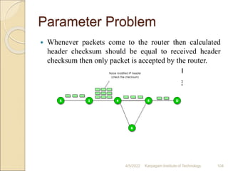
- 104. Parameter Problem Whenever packets come to the router then calculated header checksum should be equal to received header checksum then only packet is accepted by the router. 4/5/2022 Karpagam Institute of Technology 104
- 105. If there is mismatch packet will be dropped by the router. ICMP will take the source IP from the discarded packet and informs to source by sending parameter problem message. 4/5/2022 Karpagam Institute of Technology 105
- 106. Time Exceeded Message 4/5/2022 Karpagam Institute of Technology 106 When some fragments are lost in a network then the holding fragment by the router will be dropped then ICMP will take source IP from discarded packet and informs to the source, of discarded datagram due to time to live field reaches to zero, by sending time exceeded message.
- 107. Destination unreachable Destination unreachable is generated by the host or its inbound gateway to inform the client that the destination is unreachable for some reason. There is no necessary condition that only router give the ICMP error message some time destination host send ICMP error message when any type of failure (link failure,hardware failure,port failure etc) happen in the network. 4/5/2022 Karpagam Institute of Technology 107
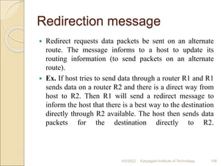
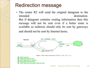
- 108. Redirection message Redirect requests data packets be sent on an alternate route. The message informs to a host to update its routing information (to send packets on an alternate route). Ex. If host tries to send data through a router R1 and R1 sends data on a router R2 and there is a direct way from host to R2. Then R1 will send a redirect message to inform the host that there is a best way to the destination directly through R2 available. The host then sends data packets for the destination directly to R2. 4/5/2022 Karpagam Institute of Technology 108
- 109. Redirection message The router R2 will send the original datagram to the intended destination. But if datagram contains routing information then this message will not be sent even if a better route is available as redirects should only be sent by gateways and should not be sent by Internet hosts. 4/5/2022 Karpagam Institute of Technology 109
- 110. ICMP Query Messages 4/5/2022 Karpagam Institute of Technology 110
- 111. ICMP Query Messages Echo Request & Reply―Combination of echo request and reply messages determines whether two systems communicate or not. Timestamp Request & Reply―Two machines can use the timestamp request and reply messages to determine the round-trip time (RTT). Address Mask Request & Reply―A host to obtain its subnet mask, sends an address mask request message to the router, which responds with an address mask reply message. Router Solicitation/Advertisement―A host broadcasts a router solicitation message to know about the router. Router broadcasts its routing information with router advertisement message. 4/5/2022 Karpagam Institute of Technology 111
- 112. ICMP MESSAGE FORMAT 4/5/2022 Karpagam Institute of Technology 112
- 113. ICMP DEBUGGING TOOLS Two tools are used for debugging purpose. They are (1) Ping (2) Traceroute 4/5/2022 Karpagam Institute of Technology 113
- 114. Ping The ping program is used to find if a host is alive and responding. The source host sends ICMP echo-request messages; the destination, if alive,responds with ICMP echo-reply messages. The ping program sets the identifier field in the echo- request and echo-reply message and starts the sequence number from 0; this number is incremented by 1 each time a new message is sent. The ping program can calculate the round-trip time. It inserts the sending time in the data section of the message. When the packet arrives, it subtracts the arrival time from the departure time to get the round-trip time (RTT). $ ping google.com 4/5/2022 Karpagam Institute of Technology 114
- 115. Traceroute or Tracert The traceroute program in UNIX or tracert in Windows can be used to trace the path of a packet from a source to the destination. It can find the IP addresses of all the routers that are visited along the path. The program is usually set to check for the maximum of 30 hops (routers) to be visited. The number of hops in the Internet is normally less than this. $ traceroute google.com 4/5/2022 Karpagam Institute of Technology 115
- 116. Routing Routing is a process which is performed by layer 3 (or network layer) devices in order to deliver the packet by choosing an optimal path from one network to another. There are 3 types of routing: 1. Static routing – Static routing is a process in which we have to manually add routes in routing table. Advantages – No routing overhead for router CPU which means a cheaper router can be used to do routing. It adds security because only administrator can allow routing to particular networks only. No bandwidth usage between routers. 4/5/2022 Karpagam Institute of Technology 116
- 117. Disadvantage – For a large network, it is a hectic task for administrator to manually add each route for the network in the routing table on each router. The administrator should have good knowledge of the topology. If a new administrator comes, then he has to manually add each route so he should have very good knowledge of the routes of the topology. 4/5/2022 Karpagam Institute of Technology 117
- 118. Default Routing This is the method where the router is configured to send all packets towards a single router (next hop). It doesn’t matter to which network the packet belongs, it is forwarded out to router which is configured for default routing. It is generally used with stub routers. A stub router is a router which has only one route to reach all other networks. 4/5/2022 Karpagam Institute of Technology 118
- 119. Dynamic Routing Dynamic routing makes automatic adjustment of the routes according to the current state of the route in the routing table. Dynamic routing uses protocols to discover network destinations and the routes to reach it. RIP and OSPF are the best examples of dynamic routing protocol. Automatic adjustment will be made to reach the network destination if one route goes down. A dynamic protocol have following features: The routers should have the same dynamic protocol running in order to exchange routes. When a router finds a change in the topology then router advertises it to all other routers. 4/5/2022 Karpagam Institute of Technology 119
- 120. Advantages – Easy to configure. More effective at selecting the best route to a destination remote network and also for discovering remote network. Disadvantage – Consumes more bandwidth for communicating with other neighbors. Less secure than static routing. 4/5/2022 Karpagam Institute of Technology 120
- 121. TYPES OF ROUTING PROTOCOLS Two types of Routing Protocols are used in the Internet: 1) Intradomain routing Routing within a single autonomous system Routing Information Protocol (RIP) - based on the distance-vector algorithm Open Shortest Path First (OSPF) - based on the link-state algorithm 2) Interdomain routing Routing between autonomous systems. Border Gateway Protocol (BGP) - based on the path-vector algorithm 4/5/2022 Karpagam Institute of Technology 121
- 122. Unicast Routing Protocols Unicast – Unicast means the transmission from a single sender to a single receiver. It is a point to point communication between sender and receiver. There are various unicast protocols such as TCP, HTTP, etc. TCP is the most commonly used unicast protocol. It is a connection oriented protocol that relay on acknowledgement from the receiver side. HTTP stands for Hyper Text Transfer Protocol. It is an object oriented protocol for communication. 4/5/2022 Karpagam Institute of Technology 122
- 123. Unicast Routing There are three main classes of routing protocols: 1) Distance Vector Routing Algorithm – Routing Information Protocol 2) Link State Routing Algorithm – Open Shortest Path First Protocol 3) Path-Vector Routing Algorithm - Border Gateway Protocol 4/5/2022 Karpagam Institute of Technology 123
- 124. DISTANCE VECTOR ROUTING (DSR) Distance vector routing is distributed, i.e., algorithm is run on all nodes. Each node knows the distance (cost) to each of its directly connected neighbors. Nodes construct a vector (Destination, Cost, NextHop) and distributes to its neighbors. Nodes compute routing table of minimum distance to every other node via NextHop using information obtained from its neighbors. 4/5/2022 Karpagam Institute of Technology 124
- 125. Initial State 4/5/2022 Karpagam Institute of Technology 125
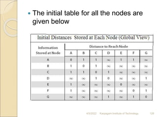
- 126. Initial State In given network, cost of each link is 1 hop. Each node sets a distance of 1 (hop) to its immediate neighbor and cost to itself as 0. Distance for non-neighbors is marked as unreachable with value ∞ (infinity). For node A, nodes B, C, E and F are reachable, whereas nodes D and G are unreachable. 4/5/2022 Karpagam Institute of Technology 126
- 127. 4/5/2022 Karpagam Institute of Technology 127
- 128. The initial table for all the nodes are given below 4/5/2022 Karpagam Institute of Technology 128
- 129. 4/5/2022 Karpagam Institute of Technology 129
- 130. 4/5/2022 Karpagam Institute of Technology 130
- 131. System stabilizes when all nodes have complete routing information, i.e., convergence. Routing tables are exchanged periodically or in case of triggered update. The final distances stored at each node is given below: 4/5/2022 Karpagam Institute of Technology 131
- 132. 4/5/2022 Karpagam Institute of Technology 132
- 133. Updation of Routing Tables There are two different circumstances under which a given node decides to send a routing update to its neighbors. 1.Periodic Update 2. Triggered Update 4/5/2022 Karpagam Institute of Technology 133
- 134. Periodic Update In this case, each node automatically sends an update message every so often, even if nothing has changed. The frequency of these periodic updates varies from protocol to protocol, but it is typically on the order of several seconds to several minutes. Triggered Update In this case, whenever a node notices a link failure or receives an update from one of its neighbors that causes it to change one of the routes in its routing table. Whenever a node’s routing table changes, it sends an update to its neighbors, which may lead to a change in their tables, causing them to send an update to their neighbors. 4/5/2022 Karpagam Institute of Technology 134
- 135. Count-To-Infinity (or) Loop Instability Problem Suppose link from node A to E goes down. Node A advertises a distance of ∞ to E to its neighbors Node B receives periodic update from C before A’s update reaches B Node B updated by C, concludes that E can be reached in 3 hops via C Node B advertises to A as 3 hops to reach E Node A in turn updates C with a distance 4/5/2022 Karpagam Institute of Technology 135
- 136. Thus nodes update each other until cost to E reaches infinity, i.e., no convergence. Routing table does not stabilize. This problem is called loop instability or count to infinity 4/5/2022 Karpagam Institute of Technology 136
- 137. Solution to Count-To-Infinity (or) Loop Instability Problem : Infinity is redefined to a small number, say 16. Distance between any two nodes can be 15 hops maximum. Thus distance vector routing cannot be used in large networks. When a node updates its neighbors, it does not send those routes it learned from each neighbor back to that neighbor. This is known as split horizon. Split horizon with poison reverse allows nodes to advertise routes it learnt from a node back to that node, but with a warning 4/5/2022 Karpagam Institute of Technology 137
- 138. ROUTING INFORMATION PROTOCOL (RIP) RIP is an intra-domain routing protocol based on distance-vector algorithm. 4/5/2022 Karpagam Institute of Technology 138
- 139. ROUTING INFORMATION PROTOCOL (RIP) Routers advertise the cost of reaching networks. Cost of reaching each link is 1hop. For example, router C advertises to A that it can reach network 2, 3 at cost 0 (directly connected), networks 5, 6 at cost 1 and network 4 at cost 2. Each router updates cost and next hop for each network number. Infinity is defined as 16, i.e., any route cannot have more than 15 hops. Therefore RIP can be implemented on small-sized networks only. Advertisements are sent every 30 seconds or in case of triggered update. 4/5/2022 Karpagam Institute of Technology 139
- 140. 4/5/2022 Karpagam Institute of Technology 140 • Command - It indicates the packet type. • Value 1 represents a request packet. Value 2 represents a response packet. • Version - It indicates the RIP version number. For RIPv1, the value is 0x01. • Address Family Identifier - When the value is 2, it represents the IP protocol. • IP Address - It indicates the destination IP address of the route. It can be the addresses of only the natural network segment. • Metric - It indicates the hop count of a route to its destination.
- 141. LINK STATE ROUTING (LSR) Each node knows state of link to its neighbors and cost. Nodes create an update packet called link-state packet (LSP) that contains: ID of the node List of neighbors for that node and associated cost 64-bit Sequence number Time to live Link-State routing protocols rely on two mechanisms: Reliable flooding of link-state information to all other nodes Route calculation from the accumulated link-state knowledge 4/5/2022 Karpagam Institute of Technology 141
- 142. Link State Routing Link state routing is a technique in which each router shares the knowledge of its neighborhood with every other router in the internetwork. The three keys to understand the Link State Routing algorithm: •Knowledge about the neighborhood: Instead of sending its routing table, a router sends the information about its neighborhood only. A router broadcast its identities and cost of the directly attached links to other routers. •Flooding: Each router sends the information to every other router on the internetwork except its neighbors. This process is known as Flooding. Every router that receives the packet sends the copies to all its neighbors. Finally, each and every router receives a copy of the same information. •Information sharing: A router sends the information to every other router only when the change occurs in the information. 4/5/2022 Karpagam Institute of Technology 142
- 143. Link state Routing Link state routing is the second family of routing protocols. While distance vector routers use a distributed algorithm to compute their routing tables, link-state routing uses link-state routers to exchange messages that allow each router to learn the entire network topology. Based on this learned topology, each router is then able to compute its routing table by using a shortest path computation. Features of link state routing protocols – Link state packet – A small packet that contains routing information. Link state database – A collection information gathered from link state packet. Shortest path first algorithm (Dijkstra algorithm) – A calculation performed on the database results into shortest path Routing table – A list of known paths and interfaces. 4/5/2022 Karpagam Institute of Technology 143
- 144. Working Principle Discover its neighbors and learn their network addresses. Measure the delay or cost to each of its neighbours. Construct a packet telling all it has just learned. Send this packet to all other routers and Compute the shortest path to every other router. 4/5/2022 Karpagam Institute of Technology 144
- 145. Step 1 Information Sharing The first step in link state routing is information sharing. Each router sends its knowledge about its neighborhood to every other router in the internetwork. 4/5/2022 Karpagam Institute of Technology 145
- 146. Step 2 Measuring Packet Cost Both distance vector and link state routing are lowest cost algorithms. In distance vector routing, cost refers to hop count. In link state routing, cost is a weighted value based on a variety of factors such as security levels, traffic or the state of the link. The cost from router A to network 1, therefore, might be different from the cost from A to network 2. Cost is applied only by routers and not by any other stations on a network. In determining a route, the cost of a hop is applied to each packet as it leaves a router and enters a network. 4/5/2022 Karpagam Institute of Technology 146
- 147. Cost in link state routing 4/5/2022 Karpagam Institute of Technology 147
- 148. Step 3 Building link state packet When a router floods the network with information about its neighbourhood, it is said to be advertising. In link state routing, a small packet containing routing information sent by the router to all other routers is referred as Link-State Packet(LSP). 4/5/2022 Karpagam Institute of Technology 148
- 149. Link State Packet Format Link- State Packet contains 4 fields The ID of the advertiser The ID of the destination network The cost The ID of the neighbor router 4/5/2022 Karpagam Institute of Technology 149
- 150. Link State Packet Format 4/5/2022 Karpagam Institute of Technology 150
- 151. Step 4: Flooding of LSP 4/5/2022 Karpagam Institute of Technology 151
- 152. Step 4: Flooding of LSP After creating LSP, every router forwards it to each and every other router in the internet. Link State Database – With the help of the information in the every LSP packet, which is received by every router and it creates a common database to all routers is referred as Link State Database. Every router stores this database on its disk, and uses it for routing packets. 4/5/2022 Karpagam Institute of Technology 152
- 153. Link State Database 4/5/2022 Karpagam Institute of Technology 153
- 154. Step 5: Computing shortest path tree Once the link state database has been created, each router applies an algorithm called Dijkstra algorithm to it, in order to calculate its routing table. 4/5/2022 Karpagam Institute of Technology 154
- 155. Shortest Path Routing 2 algorithms for computing the shorstest path between two nodes of a graph are known. 1. Dijkstra’s algorithm 2. Bellman-Ford algorithm 4/5/2022 Karpagam Institute of Technology 155
- 156. Calculation of Shortest Path To find shortest path, each node need to run the famous Dijkstra algorithm. This famous algorithm uses the following steps: Step-1: The node is taken and chosen as a root node of the tree, this creates the tree with a single node, and now set the total cost of each node to some value based on the information in Link State Database Step-2: Now the node selects one node, among all the nodes not in the tree like structure, which is nearest to the root, and adds this to the tree.The shape of the tree gets changed . Step-3: After this node is added to the tree, the cost of all the nodes not in the tree needs to be updated because the paths may have been changed. Step-4: The node repeats the Step 2. and Step 3. until all the nodes are added in the tree 4/5/2022 Karpagam Institute of Technology 156
- 157. Example 4/5/2022 Karpagam Institute of Technology 157
- 158. 4/5/2022 Karpagam Institute of Technology 158
- 159. 4/5/2022 Karpagam Institute of Technology 159
- 160. 4/5/2022 Karpagam Institute of Technology 160
- 161. Open Shortest Path First (OSPF) Protocol fundamentals Open shortest path first (OSPF) is a link-state routing protocol which is used to find the best path between the source and the destination router using its own shortest path first (SPF) algorithm. A link-state routing protocol is a protocol which uses the concept of triggered updates, i.e., if there is a change observed in the learned routing table then the updates are triggered only, not like the distance-vector routing protocol where the routing table are exchanged at a period of time. 4/5/2022 Karpagam Institute of Technology 161
- 162. It is a network layer protocol which works on the protocol number 89 and uses AD value 110. OSPF uses multicast address 224.0.0.5 for normal communication and 224.0.0.6 for update to designated router(DR)/Backup Designated Router (BDR). Criteria – To form neighbourship in OSPF, there is a criteria for both the routers: It should be present in same area Router I’d must be unique Subnet mask should be same Hello and dead timer should be same Stub flag must match Authentication must match 4/5/2022 Karpagam Institute of Technology 162
- 163. OSPF messages – OSPF messages – OSPF uses certain messages for the communication between the routers operating OSPF. Hello message – These are keep alive messages used for neighbor discovery /recovery. These are exchanged in every 10 seconds. This include following information : Router I’d, Hello/dead interval, Area I’d, Router priority, DR and BDR IP address, authentication data. Database Description (DBD) – It is the OSPF routes of the router. This contains topology of an AS or an area (routing domain). 4/5/2022 Karpagam Institute of Technology 163
- 164. OSPF messages – Link state request (LSR) – When a router receive DBD, it compares it with its own DBD. If the DBD received has some more updates than its own DBD then LSR is being sent to its neighbor. Link state update (LSU) – When a router receives LSR, it responds with LSU message containing the details requested. Link state acknowledgement – This provides reliability to the link state exchange process. It is sent as the acknowledgement of LSU. Link state advertisement (LSA) – It is an OSPF data packet that contains link-state routing information, shared only with the routers to which adjacency has been formed. 4/5/2022 Karpagam Institute of Technology 164
- 165. Timers – Hello timer – The interval in which OSPF router sends a hello message on an interface. It is 10 seconds by default. Dead timer – The interval in which the neighbor will be declared dead if it is not able to send the hello packet . It is 40 seconds by default.It is usually 4 times the hello interval but can be configured manually according to need. 4/5/2022 Karpagam Institute of Technology 165
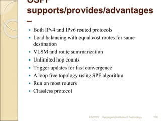
- 166. OSPF supports/provides/advantages – Both IPv4 and IPv6 routed protocols Load balancing with equal cost routes for same destination VLSM and route summarization Unlimited hop counts Trigger updates for fast convergence A loop free topology using SPF algorithm Run on most routers Classless protocol 4/5/2022 Karpagam Institute of Technology 166
- 167. Open shortest path first (OSPF) router roles – An area is a group of contiguous network and routers. Routers belonging to same area shares a common topology table and area I’d. The area I’d is associated with router’s interface as a router can belong to more than one area. There are some roles of router in OSPF: 4/5/2022 Karpagam Institute of Technology 167
- 168. OSPF 4/5/2022 Karpagam Institute of Technology 168
- 169. Area Border Router At the borders of an area, special routers are present called as area border routers, it is used to summarize the information about the area and send it to the other areas. These routers belong to both an area and the backbone. These routers are responsible for routing packets outside the area through backbone router. 4/5/2022 Karpagam Institute of Technology 169
- 170. Backbone Router Among the areas inside an autonomous system, is a special area called the backbone and the routers inside the backbone is called backbone routers. The primary role of the backbone area is to route traffic between the other areas in an AS. This router constructs a complete topological map of the entire autonomous system. 4/5/2022 Karpagam Institute of Technology 170
- 171. Boundary Routers A boundary router exchanges routing information with routers belonging to others autonomous systems 4/5/2022 Karpagam Institute of Technology 171
- 172. Internal Routers These routers are in non backbone areas and perform only intra AS routing in the area. 4/5/2022 Karpagam Institute of Technology 172
- 173. Area Summary Border Router (ASBR) – When an OSPF router is connected to a different protocol like EIGRP, or Border Gateway Protocol, or any other routing protocol then it is known as AS. The router which connects two different AS (in which one of the interface is operating OSPF) is known as Area Summary Border Router. These routers perform redistribution. ASBRs run both OSPF and another routing protocol, such as RIP or BGP. ASBRs advertise the exchanged external routing information throughout their AS. 4/5/2022 Karpagam Institute of Technology 173
- 174. OSPF terms – Router I’d – It is the highest active IP address present on the router. First, highest loopback address is considered. If no loopback is configured then the highest active IP address on the interface of the router is considered. Router priority – It is a 8 bit value assigned to a router operating OSPF, used to elect DR and BDR in a broadcast network. 4/5/2022 Karpagam Institute of Technology 174
- 175. OSPF terms – Designated Router (DR) – It is elected to minimize the number of adjacency formed. DR distributes the LSAs to all the other routers. DR is elected in a broadcast network to which all the other routers shares their DBD. In a broadcast network, router requests for an update to DR and DR will respond to that request with an update. Backup Designated Router (BDR) – BDR is backup to DR in a broadcast network. When DR goes down, BDR becomes DR and performs its functions. 4/5/2022 Karpagam Institute of Technology 175
- 176. OSPF terms – DR and BDR election – DR and BDR election takes place in broadcast network or multi-access network. Here are the criteria for the election: Router having the highest router priority will be declared as DR. If there is a tie in router priority then highest router I’d will be considered. First, the highest loopback address is considered. If no loopback is configured then the highest active IP address on the interface of the router is considered. 4/5/2022 Karpagam Institute of Technology 176
- 177. OSPF states – The device operating OSPF goes through certain states. These states are: Down – In this state, no hello packet have been received on the interface. Note – The Down state doesn’t mean that the interface is physically down. Here, it means that OSPF adjacency process has not started yet. INIT – In this state, hello packet have been received from the other router. 2WAY – In the 2WAY state, both the routers have received the hello packets from other routers. Bidirectional connectivity has been established. Note – In between the 2WAY state and Exstart state, the DR and BDR election takes place. 4/5/2022 Karpagam Institute of Technology 177
- 178. Exstart – In this state, NULL DBD are exchanged.In this state, master and slave election take place. The router having the higher router I’d becomes the master while other becomes the slave. This election decides Which router will send it’s DBD first (routers who have formed neighbourship will take part in this election). Exchange – In this state, the actual DBDs are exchanged. 4/5/2022 Karpagam Institute of Technology 178
- 179. Loading – In this sate, LSR, LSU and LSA (Link State Acknowledgement) are exchanged. Full – In this state, synchronization of all the information takes place. OSPF routing can begin only after the Full state. 4/5/2022 Karpagam Institute of Technology 179
- 180. OSPF Message Format 4/5/2022 Karpagam Institute of Technology 180
- 181. OSPF Message Format Version: It is an 8-bit field that specifies the OSPF protocol version. Type: It is an 8-bit field. It specifies the type of the OSPF packet. Message: It is a 16-bit field that defines the total length of the message, including the header. Therefore, the total length is equal to the sum of the length of the message and header. Source IP address: It defines the address from which the packets are sent. It is a sending routing IP address. Area identification: It defines the area within which the routing takes place. Checksum: It is used for error correction and error detection. Authentication type: There are two types of authentication, i.e., 0 and 1. Here, 0 means for none that specifies no authentication is available and 1 means for pwd that specifies the password-based authentication. Authentication: It is a 32-bit field that contains the actual value of the authentication data. 4/5/2022 Karpagam Institute of Technology 181
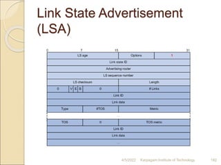
- 182. Link State Advertisement (LSA) 4/5/2022 Karpagam Institute of Technology 182
- 183. • Link state ID—ID of the router that originated the LSA. • V (Virtual Link)—Set to 1 if the router that originated the LSA is a virtual link endpoint. • E (External)—Set to 1 if the router that originated the LSA is an ASBR. • B (Border)—Set to 1 if the router that originated the LSA is an ABR. • # Links—Number of router links (interfaces) to the area, as described in the LSA. • Link ID—Determined by link type. • Link data—Determined by link type. • Type—Link type. A value of 1 indicates a point-to-point link to a remote router; a value of 2 indicates a link to a transit network; a value of 3 indicates a link to a stub network; and a value of 4 indicates a virtual link. • #TOS—Number of different TOS metrics given for this link. If no TOS metric is given for the link, this field is set to 0. TOS is not supported in RFC 2328. The #TOS field is reserved for early versions of OSPF. • Metric—Cost of using this router link. • TOS—IP Type of Service that this metric refers to. • TOS metric—TOS-specific metric information. 4/5/2022 Karpagam Institute of Technology 183
- 184. PATH VECTOR ROUTING (PVR) Path-vector routing is an asynchronous and distributed routing algorithm. The Path-vector routing is not based on least-cost routing. The best route is determined by the source using the policy it imposes on the route. In other words, the source can control the path. Path-vector routing is not actually used in an internet, and is mostly designed to route a packet between ISPs. 4/5/2022 Karpagam Institute of Technology 184
- 185. Spanning Trees In path-vector routing, the path from a source to all destinations is determined by the best spanning tree. The best spanning tree is not the least-cost tree. It is the tree determined by the source when it imposes its own policy. If there is more than one route to a destination, the source can choose the route that meets its policy best. A source may apply several policies at the same time. One of the common policies uses the minimum number of nodes to be visited. Another common policy is to avoid some nodes as 4/5/2022 Karpagam Institute of Technology 185
- 186. The spanning trees are made, gradually and asynchronously, by each node. When a node is booted, it creates a path vector based on the information it can obtain about its immediate neighbor. A node sends greeting messages to its immediate neighbors to collect these pieces of information. Each node, after the creation of the initial path vector, sends it to all its immediate neighbors. Each node, when it receives a path vector from a neighbor, updates its path vector using the formula The policy is defined by selecting the best of multiple paths. Path-vector routing also imposes one more condition on this equation. If Path (v, y) includes x, that path is discarded to avoid a loop in the path. In other words, x does not want to visit itself when it selects a path to y. 4/5/2022 Karpagam Institute of Technology 186
- 187. Example: 4/5/2022 Karpagam Institute of Technology 187
- 188. Each source has created its own spanning tree that meets its policy. The policy imposed by all sources is to use the minimum number of nodes to reach a destination. The spanning tree selected by A and E is such that the communication does not pass through D as a middle node. Similarly, the spanning tree selected by B is such that the communication does not pass through C as a middle node. 4/5/2022 Karpagam Institute of Technology 188
- 189. Path Vectors made at booting time The Figure below shows all of these path vectors for the example. Not all of these tables are created simultaneously. They are created when each node is booted. The figure also shows how these path vectors are sent to immediate neighbors after they have been created. 4/5/2022 Karpagam Institute of Technology 189
- 190. Path Vectors made at booting time 4/5/2022 Karpagam Institute of Technology 190
- 191. BORDER GATEWAY PROTOCOL (BGP) The Border Gateway Protocol version (BGP) is the only interdomain routing protocol used in the Internet today. BGP4 is based on the path-vector algorithm. It provides information about the reachability of networks in the Internet. BGP views internet as a set of autonomous systems interconnected arbitrarily. 4/5/2022 Karpagam Institute of Technology 191
- 192. BORDER GATEWAY PROTOCOL (BGP) 4/5/2022 Karpagam Institute of Technology 192
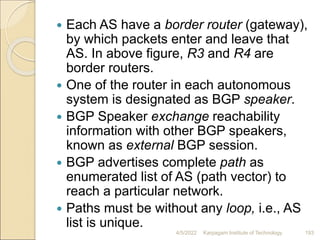
- 193. Each AS have a border router (gateway), by which packets enter and leave that AS. In above figure, R3 and R4 are border routers. One of the router in each autonomous system is designated as BGP speaker. BGP Speaker exchange reachability information with other BGP speakers, known as external BGP session. BGP advertises complete path as enumerated list of AS (path vector) to reach a particular network. Paths must be without any loop, i.e., AS list is unique. 4/5/2022 Karpagam Institute of Technology 193
- 194. For example, backbone network advertises that networks 128.96 and 192.4.153 can be reached along the path <AS1, AS2, AS4>. 4/5/2022 Karpagam Institute of Technology 194
- 195. If there are multiple routes to a destination, BGP speaker chooses one based on policy. Speakers need not advertise any route to a destination, even if one exists. Advertised paths can be cancelled, if a link/node on the path goes down. This negative advertisement is known as withdrawn route. Routes are not repeatedly sent. If there is no change, keep alive messages are sent. iBGP - interior BGP A Variant of BGP Used by routers to update routing information learnt from other speakers to routers inside the autonomous system. Each router in the AS is able to determine the appropriate next hop for all prefixes. 4/5/2022 Karpagam Institute of Technology 195
- 196. MULTICASTING 4/5/2022 Karpagam Institute of Technology 196
- 197. MULTICASTING Basic In multicasting, there is one source and a group of destinations. Multicast supports efficient delivery to multiple destinations. The relationship is one to many or many-to-many. One-to-Many (Source Specific Multicast) o Radio station broadcast o Transmitting news, stock-price o Software updates to multiple hosts Many-to-Many (Any Source Multicast) o Multimedia teleconferencing o Online multi-player games o Distributed simulations In this type of communication, the source address is a unicast address, but the destination address is a group address. The group address defines the members of the group. 4/5/2022 Karpagam Institute of Technology 197
- 198. 4/5/2022 Karpagam Institute of Technology 198
- 199. Multicasting Multicasting works in similar to Broadcasting, but in Multicasting, the information is sent to the targeted or specific members of the network. This task can be accomplished by transmitting individual copies to each user or node present in the network, but sending individual copies to each user is inefficient and might increase the network latency. To overcome these shortcomings, multicasting allows a single transmission that can be split up among the multiple users, consequently, this reduces the bandwidth of the signal. 4/5/2022 Karpagam Institute of Technology 199
- 200. Applications : Multicasting is used in many areas like: Bulk data transfer – for example, the transfer of the software upgrade from the software developer to users needing the upgrade. Internet protocol (IP) Streaming Media – for example, the transfer of the audio, video and text of the live lecture to a set of distributed lecture participants. It also supports video conferencing applications and webcasts. Data feeds Interactive gaming 4/5/2022 Karpagam Institute of Technology 200
- 201. MULTICAST ROUTING There are two types of Multicast Distribution Trees used in multicast routing. They are Source-Based Tree: (DVMRP) For each combination of (source , group), there is a shortest path spanning tree. Flood and prune Send multicast traffic everywhere Prune edges that are not actively subscribed to group Link-state Routers flood groups they would like to receive Compute shortest-path trees on demand Shared Tree (PIM) Single distributed tree shared among all sources Specify rendezvous point (RP) for group Senders send packets to RP, receivers join at RP 4/5/2022 Karpagam Institute of Technology 201
- 202. MULTICAST ROUTING PROTOCOLS Internet multicast is implemented on physical networks that support broadcasting by extending forwarding functions. Major multicast routing protocols are: 1. Distance-Vector Multicast Routing Protocol (DVMRP) 2. Protocol Independent Multicast (PIM) 4/5/2022 Karpagam Institute of Technology 202
- 203. 1. Distance Vector Multicast Routing Protocol 4/5/2022 Karpagam Institute of Technology 203
- 204. 4/5/2022 Karpagam Institute of Technology 204
- 205. Multicasting is added to distance-vector routing in four stages. Flooding Reverse Path Forwarding (RPF) Reverse Path Broadcasting (RPB) Reverse Path Multicast (RPM) 4/5/2022 Karpagam Institute of Technology 205
- 206. Flooding Router on receiving a multicast packet from source S to a Destination from NextHop, forwards the packet on all out-going links. Packet is flooded and looped back to S. The drawbacks are: 1.It floods a network, even if it has no members for that group. 2. Packets are forwarded by each router connected to a LAN, i.e., duplicate flooding 4/5/2022 Karpagam Institute of Technology 206
- 207. Reverse Path Forwarding (RPF) RPF eliminates the looping problem in the flooding process. Only one copy is forwarded and the other copies are discarded. RPF forces the router to forward a multicast packet from one specific interface: the one which has come through the shortest path from the source to the router. Packet is flooded but not looped back to S. 4/5/2022 Karpagam Institute of Technology 207
- 208. Reverse Path Forwarding (RPF) 4/5/2022 Karpagam Institute of Technology 208
- 209. Reverse-Path Broadcasting (RPB) RPB does not multicast the packet, it broadcasts it. RPB creates a shortest path broadcast tree from the source to each destination. It guarantees that each destination receives one and only one copy of the packet. We need to prevent each network from receiving more than one copy of the packet. If a network is connected to more than one router, it may receive a copy of the packet from each router. One router identified as parent called designated Router (DR). Only parent router forwards multicast packets from source S to the attached network. When a router that is not the parent of the attached network receives a multicast packet, it simply drops the packet. 4/5/2022 Karpagam Institute of Technology 209
- 210. Reverse-Path Broadcasting (RPB) 4/5/2022 Karpagam Institute of Technology 210
- 211. Reverse-Path Multicasting (RPM) To increase efficiency, the multicast packet must reach only those networks that have active members for that particular group. RPM adds pruning and grafting to RPB to create a multicast shortest path tree that supports dynamic membership changes. 4/5/2022 Karpagam Institute of Technology 211
- 212. 4/5/2022 Karpagam Institute of Technology 212
- 213. 4/5/2022 Karpagam Institute of Technology 213
- 214. Protocol Independent Multicast (PIM) 4/5/2022 Karpagam Institute of Technology 214
- 215. Example Router R4 sends Join message for group G to rendezvous router RP. Join message is received by router R2. It makes an entry (*, G) in its table and forwards the message to RP. When R5 sends Join message for group G, R2 does not forwards the Join. It adds an outgoing interface to the forwarding table created for that group. 4/5/2022 Karpagam Institute of Technology 215
- 216. 4/5/2022 Karpagam Institute of Technology 216
- 217. As routers send Join message for a group, branches are added to the tree, i.e., shared. Multicast packets sent from hosts are forwarded to designated router RP. Suppose router R1, receives a message to group G. o R1 has no state for group G. o Encapsulates the multicast packet in a Register message. o Multicast packet is tunneled along the way to RP. RP decapsulates the packet and sends multicast packet onto the shared tree, towards R2. R2 forwards the multicast packet to routers R4 4/5/2022 Karpagam Institute of Technology 217
- 218. Source-Specific Tree RP can force routers to know about group G, by sending Join message to the sending host, so that tunneling can be avoided. Intermediary routers create sender-specific entry (S, G) in their tables. Thus a source- specific route from R1 to RP is formed. If there is high rate of packets sent from a sender to a group G, then shared tree is replaced by source-specific tree with sender as root. 4/5/2022 Karpagam Institute of Technology 218
- 219. Example 4/5/2022 Karpagam Institute of Technology 219
- 220. Rendezvous router RP sends a Join message to the host router R1. Router R3 learns about group G through the message sent by RP. Router R4 send a source-specific Join due to high rate of packets from sender. Router R2 learns about group G through the message sent by R4. Eventually a source-specific tree is formed with R1 as root. 4/5/2022 Karpagam Institute of Technology 220
- 221. Analysis of PIM Protocol independent because, tree is based on Join messages via shortest path. Shared trees are more scalable than source-specific trees. Source-specific trees enable efficient routing than shared trees. 4/5/2022 Karpagam Institute of Technology 221
- 222. IPV6 - NEXT GENERATION IP IPv6 was evolved to solve address space problem and offers rich set of services. Some hosts and routers will run IPv4 only, some will run IPv4 and IPv6 and some will run IPv6 only. 4/5/2022 Karpagam Institute of Technology 222
- 223. DRAWBACKS OF IPV4 Despite subnetting and CIDR, address depletion is still a long-term problem. Internet must accommodate real-time audio and video transmission that requires minimum delay strategies and reservation of resources. Internet must provide encryption and authentication of data for some applications 4/5/2022 Karpagam Institute of Technology 223
- 224. FEATURES OF IPV6 Better header format New options Allowance for extension Support for resource allocation 4/5/2022 Karpagam Institute of Technology 224
- 225. Additional Features 1. Need to accommodate scalable routing and addressing 2. Support for real-time services 3. Security support 4. Auto configuration - The ability of hosts to automatically configure themselves with such information as their own IP address and domain name. 5. Enhanced routing functionality, including support for mobile hosts 6. Transition from ipv4 to ipv6 4/5/2022 Karpagam Institute of Technology 225
- 226. ADDRESS SPACE ALLOCATION OF IPV6 4/5/2022 Karpagam Institute of Technology 226
- 227. ADDRESS NOTATION OF IPV6 4/5/2022 Karpagam Institute of Technology 227
- 228. ADDRESS AGGREGATION OF IPV6 4/5/2022 Karpagam Institute of Technology 228
- 229. Extension Headers 4/5/2022 Karpagam Institute of Technology 229
- 230. ADVANCED CAPABILITIES OF IPV6 Auto Configuration Advanced Routing Additional Functions Security Resource allocation 4/5/2022 Karpagam Institute of Technology 230
- 231. ADVANTAGES OF IPV6 Address space ― IPv6 uses 128-bit address whereas IPv4 uses 32-bit address. Hence IPv6 has huge address space whereas IPv4 faces address shortage problem. Header format ― Unlike IPv4, optional headers are separated from base header in IPv6. Each router thus need not process unwanted addition information. Extensible ― Unassigned IPv6 addresses can accommodate needs of future technologies. 4/5/2022 Karpagam Institute of Technology 231
- 232. In IPv6 representation, we have three addressing methods : Unicast Multicast Anycast Unicast Address: Unicast Address identifies a single network interface. A packet sent to unicast address is delivered to the interface identified by that address 4/5/2022 Karpagam Institute of Technology 232
- 233. Multicast Address: Multicast Address is used by multiple hosts, called as Group, acquires a multicast destination address. These hosts need not be geographically together. If any packet is sent to this multicast address, it will be distributed to all interfaces corresponding to that multicast address. Anycast Address: Anycast Address is assigned to a group of interfaces. Any packet sent to anycast address will be delivered to only one member interface (mostly nearest host possible). 4/5/2022 Karpagam Institute of Technology 233
- 234. PACKET FORMAT OF IPV6 4/5/2022 Karpagam Institute of Technology 234
- 235. PACKET FORMAT OF IPV6 4/5/2022 Karpagam Institute of Technology 235
- 236. THANK YOU 4/5/2022 Karpagam Institute of Technology 236