


![SQL Aggregate Functions
o SQL aggregation function is used to perform the calculations on multiple rows
of a single column of a table. It returns a single value.
o It is also used to summarize the data.
Types of SQL Aggregation Function
1. COUNT FUNCTION
o COUNT function is used to Count the number of rows in a database table. It
can work on both numeric and non-numeric data types.
o COUNT function uses the COUNT(*) that returns the count of all the rows in a
specified table. COUNT(*) considers duplicate and Null.
AD
Syntax
1. COUNT(*)
2. or
3. COUNT( [ALL|DISTINCT] expression )
Sample table:
PRODUCT_MAST](https://image.slidesharecdn.com/unit3sql10-240923075331-0141bac5/85/UNIT-3-SQL-10-pdf-ORACEL-DATABASE-QUERY-OPTIMIZATION-25-320.jpg)


![2. SUM Function
Sum function is used to calculate the sum of all selected columns. It works on numeric
fields only.
Syntax
1. SUM()
2. or
3. SUM( [ALL|DISTINCT] expression )
Example: SUM()
1. SELECT SUM(COST)
2. FROM PRODUCT_MAST;
Output:
AD
670
Example: SUM() with WHERE
1. SELECT SUM(COST)
2. FROM PRODUCT_MAST
3. WHERE QTY>3;
Output:
320
Example: SUM() with GROUP BY
1. SELECT SUM(COST)
2. FROM PRODUCT_MAST
3. WHERE QTY>3
4. GROUP BY COMPANY;
Output:](https://image.slidesharecdn.com/unit3sql10-240923075331-0141bac5/85/UNIT-3-SQL-10-pdf-ORACEL-DATABASE-QUERY-OPTIMIZATION-28-320.jpg)
![Com1 150
Com2 170
Example: SUM() with HAVING
AD
1. SELECT COMPANY, SUM(COST)
2. FROM PRODUCT_MAST
3. GROUP BY COMPANY
4. HAVING SUM(COST)>=170;
Output:
Com1 335
Com3 170
3. AVG function
The AVG function is used to calculate the average value of the numeric type. AVG
function returns the average of all non-Null values.
Syntax
1. AVG()
2. or
3. AVG( [ALL|DISTINCT] expression )
Example:
1. SELECT AVG(COST)
2. FROM PRODUCT_MAST;
Output:
67.00
4. MAX Function
MAX function is used to find the maximum value of a certain column. This function
determines the largest value of all selected values of a column.](https://image.slidesharecdn.com/unit3sql10-240923075331-0141bac5/85/UNIT-3-SQL-10-pdf-ORACEL-DATABASE-QUERY-OPTIMIZATION-29-320.jpg)
![Syntax
1. MAX()
2. or
3. MAX( [ALL|DISTINCT] expression )
Example:
1. SELECT MAX(RATE)
2. FROM PRODUCT_MAST;
30
5. MIN Function
MIN function is used to find the minimum value of a certain column. This function
determines the smallest value of all selected values of a column.
Syntax
1. MIN()
2. or
3. MIN( [ALL|DISTINCT] expression )
Example:
1. SELECT MIN(RATE)
2. FROM PRODUCT_MAST;
Output:
10
Nested Sub Queries
A Subquery or Inner query or a Nested query is a query within another SQL query and
embedded within the WHERE clause.](https://image.slidesharecdn.com/unit3sql10-240923075331-0141bac5/85/UNIT-3-SQL-10-pdf-ORACEL-DATABASE-QUERY-OPTIMIZATION-30-320.jpg)
![A subquery is used to return data that will be used in the main query as a condition to further
restrict the data to be retrieved.
Subqueries can be used with the SELECT, INSERT, UPDATE, and DELETE statements along
with the operators like =, <, >, >=, <=, IN, BETWEEN, etc.
There are a few rules that subqueries must follow −
Subqueries must be enclosed within parentheses.
A subquery can have only one column in the SELECT clause, unless multiple columns
are in the main query for the subquery to compare its selected columns.
An ORDER BY command cannot be used in a subquery, although the main query can use
an ORDER BY. The GROUP BY command can be used to perform the same function as
the ORDER BY in a subquery.
Subqueries that return more than one row can only be used with multiple value operators
such as the IN operator.
The SELECT list cannot include any references to values that evaluate to a BLOB,
ARRAY, CLOB, or NCLOB.
A subquery cannot be immediately enclosed in a set function.
The BETWEEN operator cannot be used with a subquery. However, the BETWEEN
operator can be used within the subquery.
Subqueries with the SELECT Statement
Subqueries are most frequently used with the SELECT statement. The basic syntax is
as follows −
SELECT column_name [, column_name ]
FROM table1 [, table2 ]
WHERE column_name OPERATOR
(SELECT column_name [, column_name ]
FROM table1 [, table2 ]
[WHERE])
Example
Consider the CUSTOMERS table having the following records −
+----+----------+-----+-----------+----------+
| ID | NAME | AGE | ADDRESS | SALARY |
+----+----------+-----+-----------+----------+
| 1 | Ramesh | 35 | Ahmedabad | 2000.00 |
| 2 | Khilan | 25 | Delhi | 1500.00 |
| 3 | kaushik | 23 | Kota | 2000.00 |
| 4 | Chaitali | 25 | Mumbai | 6500.00 |
| 5 | Hardik | 27 | Bhopal | 8500.00 |
| 6 | Komal | 22 | MP | 4500.00 |
| 7 | Muffy | 24 | Indore | 10000.00 |
+----+----------+-----+-----------+----------+](https://image.slidesharecdn.com/unit3sql10-240923075331-0141bac5/85/UNIT-3-SQL-10-pdf-ORACEL-DATABASE-QUERY-OPTIMIZATION-31-320.jpg)
![Now, let us check the following subquery with a SELECT statement.
SQL> SELECT *
FROM CUSTOMERS
WHERE ID IN (SELECT ID
FROM CUSTOMERS
WHERE SALARY > 4500) ;
This would produce the following result.
+----+----------+-----+---------+----------+
| ID | NAME | AGE | ADDRESS | SALARY |
+----+----------+-----+---------+----------+
| 4 | Chaitali | 25 | Mumbai | 6500.00 |
| 5 | Hardik | 27 | Bhopal | 8500.00 |
| 7 | Muffy | 24 | Indore | 10000.00 |
+----+----------+-----+---------+----------+
Subqueries with the INSERT Statement
Subqueries also can be used with INSERT statements. The INSERT statement uses
the data returned from the subquery to insert into another table. The selected data in
the subquery can be modified with any of the character, date or number functions.
The basic syntax is as follows.
INSERT INTO table_name [ (column1 [, column2 ]) ]
SELECT [ *|column1 [, column2 ]
FROM table1 [, table2 ]
[ WHERE VALUE OPERATOR ]
Example
Consider a table CUSTOMERS_BKP with similar structure as CUSTOMERS table. Now to
copy the complete CUSTOMERS table into the CUSTOMERS_BKP table, you can use the
following syntax.
SQL> INSERT INTO CUSTOMERS_BKP
SELECT * FROM CUSTOMERS
WHERE ID IN (SELECT ID
FROM CUSTOMERS) ;
Subqueries with the UPDATE Statement
The subquery can be used in conjunction with the UPDATE statement. Either single or multiple
columns in a table can be updated when using a subquery with the UPDATE statement.
The basic syntax is as follows.
UPDATE table](https://image.slidesharecdn.com/unit3sql10-240923075331-0141bac5/85/UNIT-3-SQL-10-pdf-ORACEL-DATABASE-QUERY-OPTIMIZATION-32-320.jpg)
![SET column_name = new_value
[ WHERE OPERATOR [ VALUE ]
(SELECT COLUMN_NAME
FROM TABLE_NAME)
[ WHERE) ]
Example
Assuming, we have CUSTOMERS_BKP table available which is backup of CUSTOMERS
table. The following example updates SALARY by 0.25 times in the CUSTOMERS table for all
the customers whose AGE is greater than or equal to 27.
SQL> UPDATE CUSTOMERS
SET SALARY = SALARY * 0.25
WHERE AGE IN (SELECT AGE FROM CUSTOMERS_BKP
WHERE AGE >= 27 );
This would impact two rows and finally CUSTOMERS table would have the
following records.
+----+----------+-----+-----------+----------+
| ID | NAME | AGE | ADDRESS | SALARY |
+----+----------+-----+-----------+----------+
| 1 | Ramesh | 35 | Ahmedabad | 125.00 |
| 2 | Khilan | 25 | Delhi | 1500.00 |
| 3 | kaushik | 23 | Kota | 2000.00 |
| 4 | Chaitali | 25 | Mumbai | 6500.00 |
| 5 | Hardik | 27 | Bhopal | 2125.00 |
| 6 | Komal | 22 | MP | 4500.00 |
| 7 | Muffy | 24 | Indore | 10000.00 |
+----+----------+-----+-----------+----------+
Subqueries with the DELETE Statement
The subquery can be used in conjunction with the DELETE statement like with any other
statements mentioned above.
The basic syntax is as follows.
DELETE FROM TABLE_NAME
[ WHERE OPERATOR [ VALUE ]
(SELECT COLUMN_NAME
FROM TABLE_NAME)
[ WHERE) ]
Example
Assuming, we have a CUSTOMERS_BKP table available which is a backup of the
CUSTOMERS table. The following example deletes the records from the CUSTOMERS table
for all the customers whose AGE is greater than or equal to 27.](https://image.slidesharecdn.com/unit3sql10-240923075331-0141bac5/85/UNIT-3-SQL-10-pdf-ORACEL-DATABASE-QUERY-OPTIMIZATION-33-320.jpg)


![SET TRANSACTION [ READ WRITE | READ ONLY ];
Integrity Constraints
o Integrity constraints are a set of rules. It is used to maintain the quality of
information.
o Integrity constraints ensure that the data insertion, updating, and other
processes have to be performed in such a way that data integrity is not affected.
o Thus, integrity constraint is used to guard against accidental damage to the
database.
Types of Integrity Constraint](https://image.slidesharecdn.com/unit3sql10-240923075331-0141bac5/85/UNIT-3-SQL-10-pdf-ORACEL-DATABASE-QUERY-OPTIMIZATION-48-320.jpg)
UNIT 3 SQL 10.pdf ORACEL DATABASE QUERY OPTIMIZATION
- 1. UNIT 3 SQL 10 SQL Standards-Data types–structure of SQL queries–additional basic operations-set operations- null values- aggregate functions-nested sub queries-modification of the database. Intermediate SQL: Joins-Views- Transactions-Integrity constraints–Authorization. Advanced SQL. SQL Standards Oracle strives to comply with industry-accepted standards and participates actively in SQL standards committees. Industry-accepted committees are the American National Standards Institute (ANSI) and the International Organization for Standardization (ISO), which is affiliated with the International Electrotechnical Commission (IEC). Both ANSI and the ISO/IEC have accepted SQL as the standard language for relational databases. When a new SQL standard is simultaneously published by these organizations, the names of the standards conform to conventions used by the organization, but the standards are technically identical. The SQL standard consists of ten parts; one part is new in 2012; five other parts were revised in 2011; for the other four parts, the 2008 version remains in place. How SQL Works The strengths of SQL provide benefits for all types of users, including application programmers, database administrators, managers, and end users. Technically speaking, SQL is a data sublanguage. The purpose of SQL is to provide an interface to a relational database such as Oracle Database, and all SQL statements are instructions to the database. In this SQL differs from general-purpose programming languages like C and BASIC. Among the features of SQL are the following: It processes sets of data as groups rather than as individual units. It provides automatic navigation to the data. It uses statements that are complex and powerful individually, and that therefore stand alone. Flow-control statements were not part of SQL originally, but they are found in the optional part of SQL, ISO/IEC 9075-4:2011. Flow-control statements are commonly known as "persistent stored modules" (PSM), and the PL/SQL extension to Oracle SQL is similar to PSM. SQL lets you work with data at the logical level. You need to be concerned with the implementation details only when you want to manipulate the data. For example, to retrieve a set of rows from a table, you define a condition used to filter the rows. All rows satisfying the condition are retrieved in a single step and can be passed as a unit to the user, to another SQL statement, or to an application. You need not deal with the rows one by one, nor do you have to worry about how they are physically stored or retrieved. All SQL statements use the optimizer, a
- 2. part of Oracle Database that determines the most efficient means of accessing the specified data. Oracle also provides techniques that you can use to make the optimizer perform its job better. SQL provides statements for a variety of tasks, including: Querying data Inserting, updating, and deleting rows in a table Creating, replacing, altering, and dropping objects Controlling access to the database and its objects Guaranteeing database consistency and integrity SQL unifies all of the preceding tasks in one consistent language. SQL Data Types (Version 8.0) In MySQL there are three main data types: string, numeric, and date and time. String Data Types Data type Description CHAR(size) A FIXED length string (can contain letters, numbers, and special characters). The size parameter specifies the column length in characters - can be from 0 to 255. Default is 1 VARCHAR(size) A VARIABLE length string (can contain letters, numbers, and special characters). The size parameter specifies the maximum string length in characters - can be from 0 to 65535 BINARY(size) Equal to CHAR(), but stores binary byte strings. The size parameter specifies the
- 3. column length in bytes. Default is 1 VARBINARY(size) Equal to VARCHAR(), but stores binary byte strings. The size parameter specifies the maximum column length in bytes. TINYBLOB For BLOBs (Binary Large Objects). Max length: 255 bytes TINYTEXT Holds a string with a maximum length of 255 characters TEXT(size) Holds a string with a maximum length of 65,535 bytes BLOB(size) For BLOBs (Binary Large Objects). Holds up to 65,535 bytes of data MEDIUMTEXT Holds a string with a maximum length of 16,777,215 characters MEDIUMBLOB For BLOBs (Binary Large Objects). Holds up to 16,777,215 bytes of data LONGTEXT Holds a string with a maximum length of 4,294,967,295 characters LONGBLOB For BLOBs (Binary Large Objects). Holds up to 4,294,967,295 bytes of data
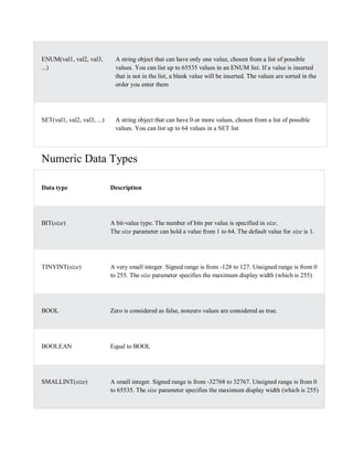
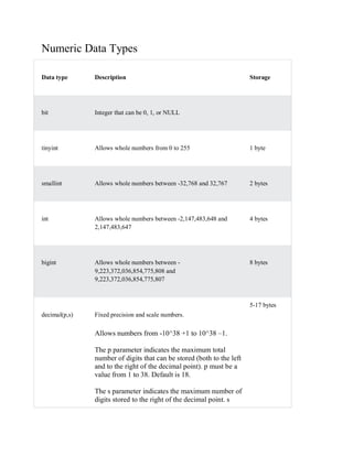
- 4. ENUM(val1, val2, val3, ...) A string object that can have only one value, chosen from a list of possible values. You can list up to 65535 values in an ENUM list. If a value is inserted that is not in the list, a blank value will be inserted. The values are sorted in the order you enter them SET(val1, val2, val3, ...) A string object that can have 0 or more values, chosen from a list of possible values. You can list up to 64 values in a SET list Numeric Data Types Data type Description BIT(size) A bit-value type. The number of bits per value is specified in size. The size parameter can hold a value from 1 to 64. The default value for size is 1. TINYINT(size) A very small integer. Signed range is from -128 to 127. Unsigned range is from 0 to 255. The size parameter specifies the maximum display width (which is 255) BOOL Zero is considered as false, nonzero values are considered as true. BOOLEAN Equal to BOOL SMALLINT(size) A small integer. Signed range is from -32768 to 32767. Unsigned range is from 0 to 65535. The size parameter specifies the maximum display width (which is 255)
- 5. MEDIUMINT(size) A medium integer. Signed range is from -8388608 to 8388607. Unsigned range is from 0 to 16777215. The size parameter specifies the maximum display width (which is 255) INT(size) A medium integer. Signed range is from -2147483648 to 2147483647. Unsigned range is from 0 to 4294967295. The size parameter specifies the maximum display width (which is 255) INTEGER(size) Equal to INT(size) BIGINT(size) A large integer. Signed range is from -9223372036854775808 to 9223372036854775807. Unsigned range is from 0 to 18446744073709551615. The size parameter specifies the maximum display width (which is 255) FLOAT(size, d) A floating point number. The total number of digits is specified in size. The number of digits after the decimal point is specified in the d parameter. This syntax is deprecated in MySQL 8.0.17, and it will be removed in future MySQL versions FLOAT(p) A floating point number. MySQL uses the p value to determine whether to use FLOAT or DOUBLE for the resulting data type. If p is from 0 to 24, the data type becomes FLOAT(). If p is from 25 to 53, the data type becomes DOUBLE() DOUBLE(size, d) A normal-size floating point number. The total number of digits is specified in size. The number of digits after the decimal point is specified in the d parameter
- 6. DOUBLE PRECISION(size, d) DECIMAL(size, d) An exact fixed-point number. The total number of digits is specified in size. The number of digits after the decimal point is specified in the d parameter. The maximum number for size is 65. The maximum number for d is 30. The default value for size is 10. The default value for d is 0. DEC(size, d) Equal to DECIMAL(size,d) Note: All the numeric data types may have an extra option: UNSIGNED or ZEROFILL. If you add the UNSIGNED option, MySQL disallows negative values for the column. If you add the ZEROFILL option, MySQL automatically also adds the UNSIGNED attribute to the column. Date and Time Data Types Data type Description DATE A date. Format: YYYY-MM-DD. The supported range is from '1000-01-01' to '9999- 12-31' DATETIME(fsp) A date and time combination. Format: YYYY-MM-DD hh:mm:ss. The supported range is from '1000-01-01 00:00:00' to '9999-12-31 23:59:59'. Adding DEFAULT and ON UPDATE in the column definition to get automatic initialization and updating to the current date and time
- 7. TIMESTAMP(fsp) A timestamp. TIMESTAMP values are stored as the number of seconds since the Unix epoch ('1970-01-01 00:00:00' UTC). Format: YYYY-MM-DD hh:mm:ss. The supported range is from '1970-01-01 00:00:01' UTC to '2038-01-09 03:14:07' UTC. Automatic initialization and updating to the current date and time can be specified using DEFAULT CURRENT_TIMESTAMP and ON UPDATE CURRENT_TIMESTAMP in the column definition TIME(fsp) A time. Format: hh:mm:ss. The supported range is from '-838:59:59' to '838:59:59' YEAR A year in four-digit format. Values allowed in four-digit format: 1901 to 2155, and 0000. MySQL 8.0 does not support year in two-digit format. SQL Server Data Types String Data Types Data type Description Max size Storage char(n) Fixed width character string 8,000 characters Defined width varchar(n) Variable width character string 8,000 characters 2 bytes + number of chars varchar(max) Variable width character string 1,073,741,824 characters 2 bytes + number of chars
- 8. text Variable width character string 2GB of text data 4 bytes + number of chars nchar Fixed width Unicode string 4,000 characters Defined width x 2 nvarchar Variable width Unicode string 4,000 characters nvarchar(max) Variable width Unicode string 536,870,912 characters ntext Variable width Unicode string 2GB of text data binary(n) Fixed width binary string 8,000 bytes varbinary Variable width binary string 8,000 bytes varbinary(max) Variable width binary string 2GB image Variable width binary string 2GB
- 9. Numeric Data Types Data type Description Storage bit Integer that can be 0, 1, or NULL tinyint Allows whole numbers from 0 to 255 1 byte smallint Allows whole numbers between -32,768 and 32,767 2 bytes int Allows whole numbers between -2,147,483,648 and 2,147,483,647 4 bytes bigint Allows whole numbers between - 9,223,372,036,854,775,808 and 9,223,372,036,854,775,807 8 bytes decimal(p,s) Fixed precision and scale numbers. Allows numbers from -10^38 +1 to 10^38 –1. The p parameter indicates the maximum total number of digits that can be stored (both to the left and to the right of the decimal point). p must be a value from 1 to 38. Default is 18. The s parameter indicates the maximum number of digits stored to the right of the decimal point. s 5-17 bytes
- 10. must be a value from 0 to p. Default value is 0 numeric(p,s) Fixed precision and scale numbers. Allows numbers from -10^38 +1 to 10^38 –1. The p parameter indicates the maximum total number of digits that can be stored (both to the left and to the right of the decimal point). p must be a value from 1 to 38. Default is 18. The s parameter indicates the maximum number of digits stored to the right of the decimal point. s must be a value from 0 to p. Default value is 0 5-17 bytes smallmoney Monetary data from -214,748.3648 to 214,748.3647 4 bytes money Monetary data from -922,337,203,685,477.5808 to 922,337,203,685,477.5807 8 bytes float(n) Floating precision number data from -1.79E + 308 to 1.79E + 308. The n parameter indicates whether the field should hold 4 or 8 bytes. float(24) holds a 4-byte field and float(53) holds an 8-byte field. Default value of n is 53. 4 or 8 bytes real Floating precision number data from -3.40E + 38 to 3.40E + 38 4 bytes Date and Time Data Types
- 11. Data type Description Storage datetime From January 1, 1753 to December 31, 9999 with an accuracy of 3.33 milliseconds 8 bytes datetime2 From January 1, 0001 to December 31, 9999 with an accuracy of 100 nanoseconds 6-8 bytes smalldatetime From January 1, 1900 to June 6, 2079 with an accuracy of 1 minute 4 bytes date Store a date only. From January 1, 0001 to December 31, 9999 3 bytes time Store a time only to an accuracy of 100 nanoseconds 3-5 bytes datetimeoffset The same as datetime2 with the addition of a time zone offset 8-10 bytes timestamp Stores a unique number that gets updated every time a row gets created or modified. The timestamp value is based upon an
- 12. internal clock and does not correspond to real time. Each table may have only one timestamp variable Other Data Types Data type Description sql_variant Stores up to 8,000 bytes of data of various data types, except text, ntext, and timestamp uniqueidentifier Stores a globally unique identifier (GUID) xml Stores XML formatted data. Maximum 2GB cursor Stores a reference to a cursor used for database operations table Stores a result-set for later processing
- 13. SQL query structure SQL includes Data Definition Language (DDL) statements and Data Manipulation Language (DML) statements. DDL statements, such as CREATE, ALTER, and DROP, modify the schema of a database. DML statements, such as SELECT, INSERT, UPDATE, and DELETE, manipulate data in tables. Most SQL queries use DML statements. When you design a DataBlade® module, consider DML statements in the abstract. DML statements can be in either of the following two forms: SELECT something FROM some table WHERE some conditions are satisfied UPDATE some table SET something WHERE some conditions are satisfied The italicized components serve different purposes in the DML query. The some table part is called “the from list” and is not important to consider when you design a DataBlade module. The something part is called “the target list” and identifies the columns for retrieval or update. The target list is the target on which the query is operating. The some conditions are satisfied part of the query is called “a qualification” because it identifies the rows that qualify to participate in the operation.When you develop a Data Blade module, consider where you expect a particular routine to be used. In the following two sections, the Data Blade module routines that typically appear in the target list and qualification are addressed. Additional Basic Operations 1. Additional operations are defined in terms of the fundamental operations. They do not add power to the algebra, but are useful to simplify common queries. 2. The Set Intersection Operation Set intersection is denoted by , and returns a relation that contains tuples that are in both of its argument relations. It does not add any power as
- 14. To find all customers having both a loan and an account at the SFU branch, we write 3. The Natural Join Operation Often we want to simplify queries on a cartesian product. For example, to find all customers having a loan at the bank and the cities in which they live, we need borrow and customer relations: Our selection predicate obtains only those tuples pertaining to only one cname. This type of operation is very common, so we have the natural join, denoted by a sign. Natural join combines a cartesian product and a selection into one operation. It performs a selection forcing equality on those attributes that appear in both relation schemes. Duplicates are removed as in all relation operations. To illustrate, we can rewrite the previous query as The resulting relation is shown in Figure 3.7. Figure 3.7: Joining borrow and customer relations. We can now make a more formal definition of natural join. o Consider and to be sets of attributes. o We denote attributes appearing in both relations by . o We denote attributes in either or both relations by . o Consider two relations and . o The natural join of and , denoted by is a relation on scheme . o It is a projection onto of a selection on where the predicate requires for each attribute in .
- 15. Formally, where . To find the assets and names of all branches which have depositors living in Stamford, we need customer, deposit and branch relations: Note that is associative. To find all customers who have both an account and a loan at the SFU branch: This is equivalent to the set intersection version we wrote earlier. We see now that there can be several ways to write a query in the relational algebra. If two relations and have no attributes in common, then , and . 4. The Division Operation Division, denoted , is suited to queries that include the phrase ``for all''. Suppose we want to find all the customers who have an account at all branches located in Brooklyn. Strategy: think of it as three steps. We can obtain the names of all branches located in Brooklyn by Figure 3.19 in the textbook shows the result. We can also find all cname, bname pairs for which the customer has an account by
- 16. Figure 3.20 in the textbook shows the result. Now we need to find all customers who appear in with every branch name in . The divide operation provides exactly those customers: which is simply . Formally, o Let and be relations. o Let . o The relation is a relation on scheme . o A tuple is in if for every tuple in there is a tuple in satisfying both of the following: o These conditions say that the portion of a tuple is in if and only if there are tuples with the portion and the portion in for every value of the portion in relation . We will look at this explanation in class more closely. The division operation can be defined in terms of the fundamental operations. Read the text for a more detailed explanation. 5. The Assignment Operation Sometimes it is useful to be able to write a relational algebra expression in parts using a temporary relation variable (as we did with and in the division example). The assignment operation, denoted , works like assignment in a programming language.
- 17. We could rewrite our division definition as No extra relation is added to the database, but the relation variable created can be used in subsequent expressions. Assignment to a permanent relation would constitute a modification to the database. SQL Set Operation The SQL Set operation is used to combine the two or more SQL SELECT statements. Types of Set Operation 1. Union 2. UnionAll 3. Intersect 4. Minus 1. Union
- 18. o The SQL Union operation is used to combine the result of two or more SQL SELECT queries. o In the union operation, all the number of datatype and columns must be same in both the tables on which UNION operation is being applied. o The union operation eliminates the duplicate rows from its resultset. Syntax 1. SELECT column_name FROM table1 2. UNION 3. SELECT column_name FROM table2; Example: The First table ID NAME 1 Jack 2 Harry 3 Jackson The Second table
- 19. ID NAME 3 Jackson 4 Stephan 5 David Union SQL query will be: 1. SELECT * FROM First 2. UNION 3. SELECT * FROM Second; The resultset table will look like: ID NAME 1 Jack 2 Harry 3 Jackson 4 Stephan 5 David 2. Union All
- 20. Union All operation is equal to the Union operation. It returns the set without removing duplication and sorting the data. Syntax: 1. SELECT column_name FROM table1 2. UNION ALL 3. SELECT column_name FROM table2; Example: Using the above First and Second table. Union All query will be like: 1. SELECT * FROM First 2. UNION ALL 3. SELECT * FROM Second; The resultset table will look like: ID NAME 1 Jack 2 Harry 3 Jackson 3 Jackson 4 Stephan 5 David
- 21. 3. Intersect o It is used to combine two SELECT statements. The Intersect operation returns the common rows from both the SELECT statements. o In the Intersect operation, the number of datatype and columns must be the same. o It has no duplicates and it arranges the data in ascending order by default. AD Syntax 1. SELECT column_name FROM table1 2. INTERSECT 3. SELECT column_name FROM table2; Example: Using the above First and Second table. Intersect query will be: 1. SELECT * FROM First 2. INTERSECT 3. SELECT * FROM Second; The resultset table will look like: AD ID NAME 3 Jackson 4. Minus
- 22. o It combines the result of two SELECT statements. Minus operator is used to display the rows which are present in the first query but absent in the second query. o It has no duplicates and data arranged in ascending order by default. Syntax: 1. SELECT column_name FROM table1 2. MINUS 3. SELECT column_name FROM table2; Example Using the above First and Second table. Minus query will be: 1. SELECT * FROM First 2. MINUS 3. SELECT * FROM Second; The resultset table will look like: AD ID NAME 1 Jack 2 Harry SQL NULL Values What is a NULL Value?
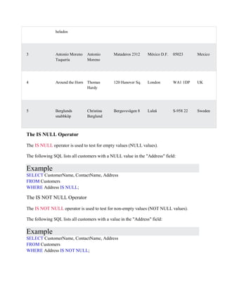
- 23. A field with a NULL value is a field with no value. If a field in a table is optional, it is possible to insert a new record or update a record without adding a value to this field. Then, the field will be saved with a NULL value. Note: A NULL value is different from a zero value or a field that contains spaces. A field with a NULL value is one that has been left blank during record creation! How to Test for NULL Values? It is not possible to test for NULL values with comparison operators, such as =, <, or <>. We will have to use the IS NULL and IS NOT NULL operators instead. IS NULL Syntax SELECT column_names FROM table_name WHERE column_name IS NULL; IS NOT NULL Syntax SELECT column_names FROM table_name WHERE column_name IS NOT NULL; Demo Database Below is a selection from the "Customers" table in the Northwind sample database: CustomerID CustomerName ContactName Address City PostalCode Country 1 Alfreds Futterkiste Maria Anders Obere Str. 57 Berlin 12209 Germany 2 Ana Trujillo Emparedados y Ana Trujillo Avda. de la Constitución 2222 México D.F. 05021 Mexico
- 24. helados 3 Antonio Moreno Taquería Antonio Moreno Mataderos 2312 México D.F. 05023 Mexico 4 Around the Horn Thomas Hardy 120 Hanover Sq. London WA1 1DP UK 5 Berglunds snabbköp Christina Berglund Berguvsvägen 8 Luleå S-958 22 Sweden The IS NULL Operator The IS NULL operator is used to test for empty values (NULL values). The following SQL lists all customers with a NULL value in the "Address" field: Example SELECT CustomerName, ContactName, Address FROM Customers WHERE Address IS NULL; The IS NOT NULL Operator The IS NOT NULL operator is used to test for non-empty values (NOT NULL values). The following SQL lists all customers with a value in the "Address" field: Example SELECT CustomerName, ContactName, Address FROM Customers WHERE Address IS NOT NULL;
- 25. SQL Aggregate Functions o SQL aggregation function is used to perform the calculations on multiple rows of a single column of a table. It returns a single value. o It is also used to summarize the data. Types of SQL Aggregation Function 1. COUNT FUNCTION o COUNT function is used to Count the number of rows in a database table. It can work on both numeric and non-numeric data types. o COUNT function uses the COUNT(*) that returns the count of all the rows in a specified table. COUNT(*) considers duplicate and Null. AD Syntax 1. COUNT(*) 2. or 3. COUNT( [ALL|DISTINCT] expression ) Sample table: PRODUCT_MAST
- 26. PRODUCT COMPANY QTY RATE COST Item1 Com1 2 10 20 Item2 Com2 3 25 75 Item3 Com1 2 30 60 Item4 Com3 5 10 50 Item5 Com2 2 20 40 Item6 Cpm1 3 25 75 Item7 Com1 5 30 150 Item8 Com1 3 10 30 Item9 Com2 2 25 50 Item10 Com3 4 30 120 Example: COUNT() 1. SELECT COUNT(*) 2. FROM PRODUCT_MAST; Output: 10 Example: COUNT with WHERE
- 27. 1. SELECT COUNT(*) 2. FROM PRODUCT_MAST; 3. WHERE RATE>=20; Output: 7 Example: COUNT() with DISTINCT 1. SELECT COUNT(DISTINCT COMPANY) 2. FROM PRODUCT_MAST; Output: 3 Example: COUNT() with GROUP BY 1. SELECT COMPANY, COUNT(*) 2. FROM PRODUCT_MAST 3. GROUP BY COMPANY; Output: Com1 5 Com2 3 Com3 2 Example: COUNT() with HAVING 1. SELECT COMPANY, COUNT(*) 2. FROM PRODUCT_MAST 3. GROUP BY COMPANY 4. HAVING COUNT(*)>2; Output: Com1 5 Com2 3
- 28. 2. SUM Function Sum function is used to calculate the sum of all selected columns. It works on numeric fields only. Syntax 1. SUM() 2. or 3. SUM( [ALL|DISTINCT] expression ) Example: SUM() 1. SELECT SUM(COST) 2. FROM PRODUCT_MAST; Output: AD 670 Example: SUM() with WHERE 1. SELECT SUM(COST) 2. FROM PRODUCT_MAST 3. WHERE QTY>3; Output: 320 Example: SUM() with GROUP BY 1. SELECT SUM(COST) 2. FROM PRODUCT_MAST 3. WHERE QTY>3 4. GROUP BY COMPANY; Output:
- 29. Com1 150 Com2 170 Example: SUM() with HAVING AD 1. SELECT COMPANY, SUM(COST) 2. FROM PRODUCT_MAST 3. GROUP BY COMPANY 4. HAVING SUM(COST)>=170; Output: Com1 335 Com3 170 3. AVG function The AVG function is used to calculate the average value of the numeric type. AVG function returns the average of all non-Null values. Syntax 1. AVG() 2. or 3. AVG( [ALL|DISTINCT] expression ) Example: 1. SELECT AVG(COST) 2. FROM PRODUCT_MAST; Output: 67.00 4. MAX Function MAX function is used to find the maximum value of a certain column. This function determines the largest value of all selected values of a column.
- 30. Syntax 1. MAX() 2. or 3. MAX( [ALL|DISTINCT] expression ) Example: 1. SELECT MAX(RATE) 2. FROM PRODUCT_MAST; 30 5. MIN Function MIN function is used to find the minimum value of a certain column. This function determines the smallest value of all selected values of a column. Syntax 1. MIN() 2. or 3. MIN( [ALL|DISTINCT] expression ) Example: 1. SELECT MIN(RATE) 2. FROM PRODUCT_MAST; Output: 10 Nested Sub Queries A Subquery or Inner query or a Nested query is a query within another SQL query and embedded within the WHERE clause.
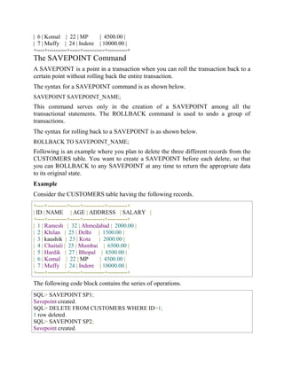
- 31. A subquery is used to return data that will be used in the main query as a condition to further restrict the data to be retrieved. Subqueries can be used with the SELECT, INSERT, UPDATE, and DELETE statements along with the operators like =, <, >, >=, <=, IN, BETWEEN, etc. There are a few rules that subqueries must follow − Subqueries must be enclosed within parentheses. A subquery can have only one column in the SELECT clause, unless multiple columns are in the main query for the subquery to compare its selected columns. An ORDER BY command cannot be used in a subquery, although the main query can use an ORDER BY. The GROUP BY command can be used to perform the same function as the ORDER BY in a subquery. Subqueries that return more than one row can only be used with multiple value operators such as the IN operator. The SELECT list cannot include any references to values that evaluate to a BLOB, ARRAY, CLOB, or NCLOB. A subquery cannot be immediately enclosed in a set function. The BETWEEN operator cannot be used with a subquery. However, the BETWEEN operator can be used within the subquery. Subqueries with the SELECT Statement Subqueries are most frequently used with the SELECT statement. The basic syntax is as follows − SELECT column_name [, column_name ] FROM table1 [, table2 ] WHERE column_name OPERATOR (SELECT column_name [, column_name ] FROM table1 [, table2 ] [WHERE]) Example Consider the CUSTOMERS table having the following records − +----+----------+-----+-----------+----------+ | ID | NAME | AGE | ADDRESS | SALARY | +----+----------+-----+-----------+----------+ | 1 | Ramesh | 35 | Ahmedabad | 2000.00 | | 2 | Khilan | 25 | Delhi | 1500.00 | | 3 | kaushik | 23 | Kota | 2000.00 | | 4 | Chaitali | 25 | Mumbai | 6500.00 | | 5 | Hardik | 27 | Bhopal | 8500.00 | | 6 | Komal | 22 | MP | 4500.00 | | 7 | Muffy | 24 | Indore | 10000.00 | +----+----------+-----+-----------+----------+
- 32. Now, let us check the following subquery with a SELECT statement. SQL> SELECT * FROM CUSTOMERS WHERE ID IN (SELECT ID FROM CUSTOMERS WHERE SALARY > 4500) ; This would produce the following result. +----+----------+-----+---------+----------+ | ID | NAME | AGE | ADDRESS | SALARY | +----+----------+-----+---------+----------+ | 4 | Chaitali | 25 | Mumbai | 6500.00 | | 5 | Hardik | 27 | Bhopal | 8500.00 | | 7 | Muffy | 24 | Indore | 10000.00 | +----+----------+-----+---------+----------+ Subqueries with the INSERT Statement Subqueries also can be used with INSERT statements. The INSERT statement uses the data returned from the subquery to insert into another table. The selected data in the subquery can be modified with any of the character, date or number functions. The basic syntax is as follows. INSERT INTO table_name [ (column1 [, column2 ]) ] SELECT [ *|column1 [, column2 ] FROM table1 [, table2 ] [ WHERE VALUE OPERATOR ] Example Consider a table CUSTOMERS_BKP with similar structure as CUSTOMERS table. Now to copy the complete CUSTOMERS table into the CUSTOMERS_BKP table, you can use the following syntax. SQL> INSERT INTO CUSTOMERS_BKP SELECT * FROM CUSTOMERS WHERE ID IN (SELECT ID FROM CUSTOMERS) ; Subqueries with the UPDATE Statement The subquery can be used in conjunction with the UPDATE statement. Either single or multiple columns in a table can be updated when using a subquery with the UPDATE statement. The basic syntax is as follows. UPDATE table
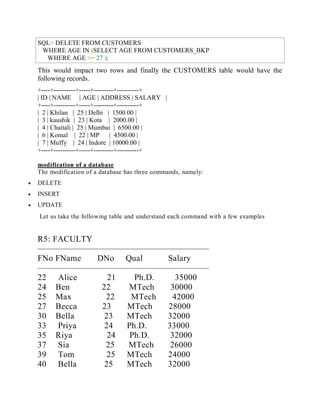
- 33. SET column_name = new_value [ WHERE OPERATOR [ VALUE ] (SELECT COLUMN_NAME FROM TABLE_NAME) [ WHERE) ] Example Assuming, we have CUSTOMERS_BKP table available which is backup of CUSTOMERS table. The following example updates SALARY by 0.25 times in the CUSTOMERS table for all the customers whose AGE is greater than or equal to 27. SQL> UPDATE CUSTOMERS SET SALARY = SALARY * 0.25 WHERE AGE IN (SELECT AGE FROM CUSTOMERS_BKP WHERE AGE >= 27 ); This would impact two rows and finally CUSTOMERS table would have the following records. +----+----------+-----+-----------+----------+ | ID | NAME | AGE | ADDRESS | SALARY | +----+----------+-----+-----------+----------+ | 1 | Ramesh | 35 | Ahmedabad | 125.00 | | 2 | Khilan | 25 | Delhi | 1500.00 | | 3 | kaushik | 23 | Kota | 2000.00 | | 4 | Chaitali | 25 | Mumbai | 6500.00 | | 5 | Hardik | 27 | Bhopal | 2125.00 | | 6 | Komal | 22 | MP | 4500.00 | | 7 | Muffy | 24 | Indore | 10000.00 | +----+----------+-----+-----------+----------+ Subqueries with the DELETE Statement The subquery can be used in conjunction with the DELETE statement like with any other statements mentioned above. The basic syntax is as follows. DELETE FROM TABLE_NAME [ WHERE OPERATOR [ VALUE ] (SELECT COLUMN_NAME FROM TABLE_NAME) [ WHERE) ] Example Assuming, we have a CUSTOMERS_BKP table available which is a backup of the CUSTOMERS table. The following example deletes the records from the CUSTOMERS table for all the customers whose AGE is greater than or equal to 27.
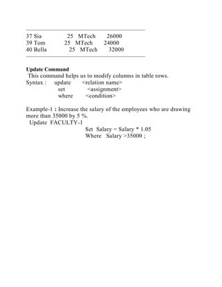
- 34. SQL> DELETE FROM CUSTOMERS WHERE AGE IN (SELECT AGE FROM CUSTOMERS_BKP WHERE AGE >= 27 ); This would impact two rows and finally the CUSTOMERS table would have the following records. +----+----------+-----+---------+----------+ | ID | NAME | AGE | ADDRESS | SALARY | +----+----------+-----+---------+----------+ | 2 | Khilan | 25 | Delhi | 1500.00 | | 3 | kaushik | 23 | Kota | 2000.00 | | 4 | Chaitali | 25 | Mumbai | 6500.00 | | 6 | Komal | 22 | MP | 4500.00 | | 7 | Muffy | 24 | Indore | 10000.00 | +----+----------+-----+---------+----------+ modification of a database The modification of a database has three commands, namely: DELETE INSERT UPDATE Let us take the following table and understand each command with a few examples R5: FACULTY ———————————————————— FNo FName DNo Qual Salary ———————————————————— 22 Alice 21 Ph.D. 35000 24 Ben 22 MTech 30000 25 Max 22 MTech 42000 27 Becca 23 MTech 28000 30 Bella 23 MTech 32000 33 Priya 24 Ph.D. 33000 35 Riya 24 Ph.D. 32000 37 Sia 25 MTech 26000 39 Tom 25 MTech 24000 40 Bella 25 MTech 32000
- 35. ———————————————————— Delete Command This command helps us to remove rows from the table. Syntax : DELETE from r where P Example-1: Remove all the employees from Dept. no 24. DELETE From FACULTY-1 Where DNo = 24 ; Output : There will be 8 tuples left in Faculty-1. Example-2 : Remove all the employees from ECE Dept. DELETE From FACULTY-1 Where DNo = (Select DNo From DEPT Where DName = ‘ECE’ ) ; Output : There will be 8 tuples left in Faculty-1. Example-3 : Remove all the employees whose salary is less than 30000. Delete From FACULTY-1 Where Salary< 30000 ; Output : There will be 7 tuples left in Faculty-1. Example-4 : Remove all the employees whose salary is less than the average salary of all the employees. Delete From FACULTY-1 Where Salary< (Select avg(Salary)
- 36. From FACULTY-1) ; Output : FNo FName DNo Qual Salary ———————————————————— 22 Alice 21 Ph.D. 35000 25 Max 22 MTech 42000 30 Bella 23 MTech 32000 33 Priya 24 Ph.D. 33000 35 Riya 24 Ph.D. 32000 40 Bella 25 MTech 34000 Note : The average salary is : 31,600 Insert Command This command helps us to insert rows into the table. Syntax : INSERT into relation-name values (…..) Example-1 : Add a tuple to FACULTY-1. Insert into FACULTY-1 values (532, ‘XX’, 28,’MTech’,25000) ; Example-2 :Add a tuple to STUD relation Insert into STUD values ( 130, ‘def’, 24) ; Example-3 :select tuples from FACULTY-1 and create a relation FACULTY-2 with tuples belonging to DNo 25. Let’s assume table structure for FACULTY-2 is already there. Insert into FACULTY-2 (Select FNo, FName, DNo, Qual, Salary From FACULTY-1 Where DNo = 25) ; R5 : FACULTY-2 ———————————————————— FNo FName DNo Qual Salary
- 37. ———————————————————— 37 Sia 25 MTech 26000 39 Tom 25 MTech 24000 40 Bella 25 MTech 32000 ———————————————————— Update Command This command helps us to modify columns in table rows. Syntax : update <relation name> set <assignment> where <condition> Example-1 : Increase the salary of the employees who are drawing more than 35000 by 5 %. Update FACULTY-1 Set Salary = Salary * 1.05 Where Salary >35000 ;
- 38. SQL | Views Views in SQL are kind of virtual tables. A view also has rows and columns as they are in a real table in the database. We can create a view by selecting fields from one or more tables present in the database. A View can either have all the rows of a table or specific rows based on certain condition we will learn about creating , deleting and updating Views. Sample Tables: StudentDetails StudentMarks CREATING VIEWS We can create View using CREATE VIEW statement. A View can be created from a single table or multiple tables. Syntax: CREATE VIEW view_name AS SELECT column1, column2..... FROM table_name WHERE condition; view_name: Name for the View table_name: Name of the table condition: Condition to select rows Examples: Creating View from a single table: In this example we will create a View named DetailsView from the table StudentDetails. Query: CREATE VIEW DetailsView AS SELECT NAME, ADDRESS
- 39. FROM StudentDetails WHERE S_ID < 5; To see the data in the View, we can query the view in the same manner as we query a table. SELECT * FROM DetailsView; Output: In this example, we will create a view named StudentNames from the table StudentDetails. Query: CREATE VIEW StudentNames AS SELECT S_ID, NAME FROM StudentDetails ORDER BY NAME; If we now query the view as, SELECT * FROM StudentNames; Output: Creating View from multiple tables: In this example we will create a View named MarksView from two tables StudentDetails and StudentMarks. To create a View from multiple tables we can simply include multiple tables in the SELECT statement. Query: CREATE VIEW MarksView AS SELECT StudentDetails.NAME, StudentDetails.ADDRESS, StudentMarks.MARKS FROM StudentDetails, StudentMarks WHERE StudentDetails.NAME = StudentMarks.NAME; To display data of View MarksView:
- 40. SELECT * FROM MarksView; Output: DELETING VIEWS We have learned about creating a View, but what if a created View is not needed any more? Obviously we will want to delete it. SQL allows us to delete an existing View. We can delete or drop a View using the DROP statement. Syntax: DROP VIEW view_name; view_name: Name of the View which we want to delete. For example, if we want to delete the View MarksView, we can do this as: DROP VIEW MarksView; UPDATING VIEWS There are certain conditions needed to be satisfied to update a view. If any one of these conditions is not met, then we will not be allowed to update the view. The SELECT statement which is used to create the view should not include GROUP BY clause or ORDER BY clause. The SELECT statement should not have the DISTINCT keyword. The View should have all NOT NULL values. The view should not be created using nested queries or complex queries. The view should be created from a single table. If the view is created using multiple tables then we will not be allowed to update the view. We can use the CREATE OR REPLACE VIEW statement to add or remove fields from a view. Syntax: CREATE OR REPLACE VIEW view_name AS SELECT column1,column2,.. FROM table_name WHERE condition; For example, if we want to update the view MarksView and add the field AGE to this View from StudentMarks Table, we can do this as: CREATE OR REPLACE VIEW MarksView AS SELECT StudentDetails.NAME, StudentDetails.ADDRESS, StudentMarks.MARKS, StudentMarks.AGE FROM StudentDetails, StudentMarks WHERE StudentDetails.NAME = StudentMarks.NAME;
- 41. If we fetch all the data from MarksView now as: SELECT * FROM MarksView; Output: Inserting a row in a view: We can insert a row in a View in a same way as we do in a table. We can use the INSERT INTO statement of SQL to insert a row in a View.Syntax: INSERT INTO view_name(column1, column2 , column3,..) VALUES(value1, value2, value3..); view_name: Name of the View Example: In the below example we will insert a new row in the View DetailsView which we have created above in the example of “creating views from a single table”. INSERT INTO DetailsView(NAME, ADDRESS) VALUES("Suresh","Gurgaon"); If we fetch all the data from DetailsView now as, SELECT * FROM DetailsView; Output: Deleting a row from a View: Deleting rows from a view is also as simple as deleting rows from a table. We can use the DELETE statement of SQL to delete rows from a view. Also deleting a row from a view first delete the row from the actual table and the change is then reflected in the view. Syntax: DELETE FROM view_name
- 42. WHERE condition; view_name:Name of view from where we want to delete rows condition: Condition to select rows Example: In this example we will delete the last row from the view DetailsView which we just added in the above example of inserting rows. DELETE FROM DetailsView WHERE NAME="Suresh"; If we fetch all the data from DetailsView now as, SELECT * FROM DetailsView; Output: WITH CHECK OPTION The WITH CHECK OPTION clause in SQL is a very useful clause for views. It is applicable to a updatable view. If the view is not updatable, then there is no meaning of including this clause in the CREATE VIEW statement. The WITH CHECK OPTION clause is used to prevent the insertion of rows in the view where the condition in the WHERE clause in CREATE VIEW statement is not satisfied. If we have used the WITH CHECK OPTION clause in the CREATE VIEW statement, and if the UPDATE or INSERT clause does not satisfy the conditions then they will return an error. Example: In the below example we are creating a View SampleView from StudentDetails Table with WITH CHECK OPTION clause. CREATE VIEW SampleView AS SELECT S_ID, NAME FROM StudentDetails WHERE NAME IS NOT NULL WITH CHECK OPTION; SQL – Transactions A transaction is a unit of work that is performed against a database. Transactions are units or sequences of work accomplished in a logical order, whether in a manual fashion by a user or automatically by some sort of a database program.
- 43. A transaction is the propagation of one or more changes to the database. For example, if you are creating a record or updating a record or deleting a record from the table, then you are performing a transaction on that table. It is important to control these transactions to ensure the data integrity and to handle database errors. Practically, you will club many SQL queries into a group and you will execute all of them together as a part of a transaction. Properties of Transactions Transactions have the following four standard properties, usually referred to by the acronym ACID. Atomicity − ensures that all operations within the work unit are completed successfully. Otherwise, the transaction is aborted at the point of failure and all the previous operations are rolled back to their former state. Consistency − ensures that the database properly changes states upon a successfully committed transaction. Isolation − enables transactions to operate independently of and transparent to each other. Durability − ensures that the result or effect of a committed transaction persists in case of a system failure. Transaction Control The following commands are used to control transactions. COMMIT − to save the changes. ROLLBACK − to roll back the changes. SAVEPOINT − creates points within the groups of transactions in which to ROLLBACK. SET TRANSACTION − Places a name on a transaction. Transactional Control Commands Transactional control commands are only used with the DML Commands such as - INSERT, UPDATE and DELETE only. They cannot be used while creating tables or dropping them because these operations are automatically committed in the database. The COMMIT Command The COMMIT command is the transactional command used to save changes invoked by a transaction to the database.
- 44. The COMMIT command is the transactional command used to save changes invoked by a transaction to the database. The COMMIT command saves all the transactions to the database since the last COMMIT or ROLLBACK command. The syntax for the COMMIT command is as follows. COMMIT; Example Consider the CUSTOMERS table having the following records − +----+----------+-----+-----------+----------+ | ID | NAME | AGE | ADDRESS | SALARY | +----+----------+-----+-----------+----------+ | 1 | Ramesh | 32 | Ahmedabad | 2000.00 | | 2 | Khilan | 25 | Delhi | 1500.00 | | 3 | kaushik | 23 | Kota | 2000.00 | | 4 | Chaitali | 25 | Mumbai | 6500.00 | | 5 | Hardik | 27 | Bhopal | 8500.00 | | 6 | Komal | 22 | MP | 4500.00 | | 7 | Muffy | 24 | Indore | 10000.00 | +----+----------+-----+-----------+----------+ Following is an example which would delete those records from the table which have age = 25 and then COMMIT the changes in the database. SQL> DELETE FROM CUSTOMERS WHERE AGE = 25; SQL> COMMIT; Thus, two rows from the table would be deleted and the SELECT statement would produce the following result. +----+----------+-----+-----------+----------+ | ID | NAME | AGE | ADDRESS | SALARY | +----+----------+-----+-----------+----------+ | 1 | Ramesh | 32 | Ahmedabad | 2000.00 | | 3 | kaushik | 23 | Kota | 2000.00 | | 5 | Hardik | 27 | Bhopal | 8500.00 | | 6 | Komal | 22 | MP | 4500.00 |
- 45. | 7 | Muffy | 24 | Indore | 10000.00 | +----+----------+-----+-----------+----------+ The ROLLBACK Command The ROLLBACK command is the transactional command used to undo transactions that have not already been saved to the database. This command can only be used to undo transactions since the last COMMIT or ROLLBACK command was issued. The syntax for a ROLLBACK command is as follows − ROLLBACK; Example Consider the CUSTOMERS table having the following records − +----+----------+-----+-----------+----------+ | ID | NAME | AGE | ADDRESS | SALARY | +----+----------+-----+-----------+----------+ | 1 | Ramesh | 32 | Ahmedabad | 2000.00 | | 2 | Khilan | 25 | Delhi | 1500.00 | | 3 | kaushik | 23 | Kota | 2000.00 | | 4 | Chaitali | 25 | Mumbai | 6500.00 | | 5 | Hardik | 27 | Bhopal | 8500.00 | | 6 | Komal | 22 | MP | 4500.00 | | 7 | Muffy | 24 | Indore | 10000.00 | +----+----------+-----+-----------+----------+ Following is an example, which would delete those records from the table which have the age = 25 and then ROLLBACK the changes in the database. SQL> DELETE FROM CUSTOMERS WHERE AGE = 25; SQL> ROLLBACK; Thus, the delete operation would not impact the table and the SELECT statement would produce the following result. +----+----------+-----+-----------+----------+ | ID | NAME | AGE | ADDRESS | SALARY | +----+----------+-----+-----------+----------+ | 1 | Ramesh | 32 | Ahmedabad | 2000.00 | | 2 | Khilan | 25 | Delhi | 1500.00 | | 3 | kaushik | 23 | Kota | 2000.00 | | 4 | Chaitali | 25 | Mumbai | 6500.00 | | 5 | Hardik | 27 | Bhopal | 8500.00 |
- 46. | 6 | Komal | 22 | MP | 4500.00 | | 7 | Muffy | 24 | Indore | 10000.00 | +----+----------+-----+-----------+----------+ The SAVEPOINT Command A SAVEPOINT is a point in a transaction when you can roll the transaction back to a certain point without rolling back the entire transaction. The syntax for a SAVEPOINT command is as shown below. SAVEPOINT SAVEPOINT_NAME; This command serves only in the creation of a SAVEPOINT among all the transactional statements. The ROLLBACK command is used to undo a group of transactions. The syntax for rolling back to a SAVEPOINT is as shown below. ROLLBACK TO SAVEPOINT_NAME; Following is an example where you plan to delete the three different records from the CUSTOMERS table. You want to create a SAVEPOINT before each delete, so that you can ROLLBACK to any SAVEPOINT at any time to return the appropriate data to its original state. Example Consider the CUSTOMERS table having the following records. +----+----------+-----+-----------+----------+ | ID | NAME | AGE | ADDRESS | SALARY | +----+----------+-----+-----------+----------+ | 1 | Ramesh | 32 | Ahmedabad | 2000.00 | | 2 | Khilan | 25 | Delhi | 1500.00 | | 3 | kaushik | 23 | Kota | 2000.00 | | 4 | Chaitali | 25 | Mumbai | 6500.00 | | 5 | Hardik | 27 | Bhopal | 8500.00 | | 6 | Komal | 22 | MP | 4500.00 | | 7 | Muffy | 24 | Indore | 10000.00 | +----+----------+-----+-----------+----------+ The following code block contains the series of operations. SQL> SAVEPOINT SP1; Savepoint created. SQL> DELETE FROM CUSTOMERS WHERE ID=1; 1 row deleted. SQL> SAVEPOINT SP2; Savepoint created.
- 47. SQL> DELETE FROM CUSTOMERS WHERE ID=2; 1 row deleted. SQL> SAVEPOINT SP3; Savepoint created. SQL> DELETE FROM CUSTOMERS WHERE ID=3; 1 row deleted. Now that the three deletions have taken place, let us assume that you have changed your mind and decided to ROLLBACK to the SAVEPOINT that you identified as SP2. Because SP2 was created after the first deletion, the last two deletions are undone − SQL> ROLLBACK TO SP2; Rollback complete. Notice that only the first deletion took place since you rolled back to SP2. SQL> SELECT * FROM CUSTOMERS; +----+----------+-----+-----------+----------+ | ID | NAME | AGE | ADDRESS | SALARY | +----+----------+-----+-----------+----------+ | 2 | Khilan | 25 | Delhi | 1500.00 | | 3 | kaushik | 23 | Kota | 2000.00 | | 4 | Chaitali | 25 | Mumbai | 6500.00 | | 5 | Hardik | 27 | Bhopal | 8500.00 | | 6 | Komal | 22 | MP | 4500.00 | | 7 | Muffy | 24 | Indore | 10000.00 | +----+----------+-----+-----------+----------+ 6 rows selected. The RELEASE SAVEPOINT Command The RELEASE SAVEPOINT command is used to remove a SAVEPOINT that you have created. The syntax for a RELEASE SAVEPOINT command is as follows. RELEASE SAVEPOINT SAVEPOINT_NAME; Once a SAVEPOINT has been released, you can no longer use the ROLLBACK command to undo transactions performed since the last SAVEPOINT. The SET TRANSACTION Command The SET TRANSACTION command can be used to initiate a database transaction. This command is used to specify characteristics for the transaction that follows. For example, you can specify a transaction to be read only or read write. The syntax for a SET TRANSACTION command is as follows.
- 48. SET TRANSACTION [ READ WRITE | READ ONLY ]; Integrity Constraints o Integrity constraints are a set of rules. It is used to maintain the quality of information. o Integrity constraints ensure that the data insertion, updating, and other processes have to be performed in such a way that data integrity is not affected. o Thus, integrity constraint is used to guard against accidental damage to the database. Types of Integrity Constraint