Unit - i-Image Transformations Gonzalez.ppt

1
UNIT-1:

Image Transformations

CONTENTS
 Need for Image Transforms, Spatial Frequencies in
Image Processing
 Introduction to Fourier Transform, Discrete Fourier
Transform, Fast Fourier Transform and its algorithm
 Properties of Fourier transform
 Discrete Cosine Transform
 Discrete Sine Transform
 Walsh Transform, Hadamard Transform
 Haar Transform, Slant Transform
 SVD and KLTransforms or Hotelling Transform
2

3
Introduction
 Definition: Image transform = operation to
change the default representation space of a
digital image (spatial domain -> another domain)
so that:
 all the information present in the image is
preserved in the transformed domain, but
represented differently;
 the transform is reversible, i.e., we can revert to
the spatial domain

Need for transform
 Mathematical convenience
 To explore more details
 Critical image components are
isolated so that user can directly deal
with it
 Compact form of representation to
store and transmit
4

5
Fourier Transform (1-D)
       
   
 
uX
uX
sin
AX
u
F
e
uX
sin
u
A
dx
ux
2
j
exp
x
f
u
F uX
j









 






6
Fourier Transform (2-D)
   
     
 
 
 
vY
vY
sin
uX
uX
sin
AXY
v
,
u
F
dy
dx
vy
ux
2
j
exp
y
,
x
f
)
v
,
u
(
F









 







7
Discrete Fourier Transform
In the two-variable case the discrete Fourier transform pair is

8
When images are sampled in a squared array, i.e. M=N,
we can write

9
Discrete
Fourier
Transform
Examples
At all of these
examples, the Fourier
spectrum is shifted
from top left corner to
the center of the
frequency square.

10
Discrete
Fourier
Transform
Examples
At all of these
spectrum is shifted
the center of the
frequency square.

11
Discrete
Fourier
Transform
Display
At all of these
spectrum is shifted
the center of the
frequency square.

12
Example
Main Image (Gray Level) DFT of Main image
(Fourier spectrum)
Logarithmic scaled
of the Fourier spectrum

13
(Properties)
 Separability
The discrete Fourier transform pair can be expressed in the seperable forms:
       
       




















1
N
0
v
1
N
0
u
1
N
0
y
1
N
0
x
N
/
vy
2
j
exp
v
,
u
F
N
/
ux
2
j
exp
N
1
y
,
x
f
N
/
vy
2
j
exp
y
,
x
f
N
/
ux
2
j
exp
N
1
v
,
u
F

14
(Properties)
 Translation
   
   
     
 
N
/
vy
ux
2
j
exp
v
,
u
F
y
y
,
x
x
f
and
v
v
,
u
u
F
N
/
y
v
x
u
2
j
exp
y
,
x
f
0
0
0
0
0
0
0
0











The translation properties of the
Fourier transform pair are :

15
(Properties)
 Periodicity
The discrete Fourier transform and its
inverse are periodic with period N; that is,
F(u,v)=F(u+N,v)=F(u,v+N)=F(u+N,v+N)
If f(x,y) is real, the Fourier transform also
exhibits conjugate symmetry:
F(u,v)=F*
(-u,-v)
Or, more interestingly:
|F(u,v)|=|F(-u,-v)|

16
(Properties)
 Rotation
If we introduce the polar coordinates










sin
v
cos
u
sin
r
y
cos
r
x
Then we can write:
   
0
0 ,
F
,
r
f 







In other words, rotating F(u,v)
rotates f(x,y) by the same angle.

17
(Properties)
 Convolution
The convolution theorem in
two dimensions is expressed
by the relations :
     
       
v
,
u
G
*
v
,
u
F
y
,
x
g
y
,
x
f
and
v
,
u
G
v
,
u
F
)
y
,
x
(
g
*
y
,
x
f


Note :
       















 d
d
y
,
x
g
,
f
y
,
x
g
*
y
,
x
f

18
(Properties)
 Correlation
The correlation of two continuous
functions f(x) and g(x) is defined
by the relation
        







d
x
g
f
x
g
x
f *

So we can write:
       
       
v
,
u
G
v
,
u
F
y
,
x
g
y
,
x
f
and
v
,
u
G
v
,
u
F
y
,
x
g
y
,
x
f
*
*





19
Discrete
Fourier
Transform
 Sampling
(Properties)
1-D
The Fourier transform and the convolution theorem provide the
tools for a deeper analytic study of sampling problem. In particular, we
want to look at the question of how many samples should be taken so that
no information is lost in the sampling process. Expressed differently, the
problem is one of the establishing the sampling conditions under which a
continuous image can be recovered fully from a set of sampled values. We
begin the analysis with the 1-D case.
As a result, a function which is band-limited in frequency domain
must extend from negative infinity to positive infinity in time domain (or x
domain).

20
Discrete
Fourier
Transform
 Sampling
(Properties)
1-D
f(x) : a given function
F(u): Fourier Transform of f(x)
which is band-limited
s(x) : sampling function
S(u): Fourier Transform of s(x)
G(u): window for recovery of
the main function F(u) and f(x).
Recovered f(x) from sampled data

21
Discrete
Fourier
Transform
 Sampling
(Properties)
1-D
f(x) : a given function
F(u): Fourier Transform of f(x)
which is band-limited
s(x) : sampling function
S(u): Fourier Transform of s(x)
h(x): window for making f(x)
finited in time.
H(u): Fourier Transform of h(x)

22
Discrete
Fourier
Transform
 Sampling
(Properties)
1-D
s(x)*f(x) (convolution
function) is periodic, with
period 1/Δu. If N samples of
f(x) and F(u) are taken and the
spacings between samples are
selected so that a period in
each domain is covered by N
uniformly spaced samples,
then NΔx=X in the x domain
and NΔu=1/Δx in the
frequency domain.

23
Discrete
Fourier
Transform
 Sampling
(Properties)
2-D
The sampling process for 2-D
functions can be formulated
mathematically by making use
of the 2-D impulse function
δ(x,y), which is defined as
     
0
0
0
0 y
,
x
f
dy
dx
y
y
,
x
x
y
,
x
f 










A 2-D sampling function is
consisted of a train of impulses
separated Δx units in the x
direction and Δy units in the y
direction as shown in the figure.

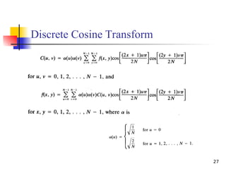
24
Discrete
Fourier
Transform
 Sampling
(Properties)
2-D
If f(x,y) is band limited (that is, its
Fourier transform vanishes outside
some finite region R) the result of
covolving S(u,v) and F(u,v) might
look like the case in the case
shown in the figure. The function
shown is periodic in two
dimensions.
 








0
1
v
,
u
G
(u,v) inside one of the rectangles
enclosing R
elsewhere
The inverse Fourier transform of
G(u,v)[S(u,v)*F(u,v)] yields f(x,y).

25
The Fast Fourier Transform (FFT) Algorithm

Discrete Sine Transform (DST)
26
 The discrete Sine transform (DST):
v(k,l)
2
N 1
u(m,n) sin
(m 1)(k 1)
N 1
sin
(n 1)(l 1)
N 1
n 0
N 1
m 0
N 1



 







 













 
(4.52)
u(m,n)
2
N 1
v(k,l) sin
(m 1)(k 1)
N 1
sin
(n 1)(l 1)
N 1
l 0
N 1
k 0
N 1



 







 













 
(4.53)
s
2
N 1
sin
(m 1)(k 1)
N 1
m,k 

 








(4.54)
 The Hartley transform:
v(k,l)
1
N
u(m,n)cas
2
N
(mk nl)
n 0
N 1
m 0
N 1
 













(4.55)
u m n
( , )  












1
N
v(k,l)cas
2
N
(mk nl)
l 0
N 1
k 0
N 1

(4.56)
cas( ) cos( ) sin( ) 2cos( / 4)
    
    (4.57)
h
1
N
m,k 












cas
mk
N
2 (4.58)

28
Discrete Cosine Transform (DCT)
Each block consists
of 4×4 elements,
corresponding to x
and y varying from 0
to 3. The highest
value is shown in
white. Other values
are shown in grays,
with darker meaning
smaller.

29
Discrete Cosine Transform
Example
Main Image (Gray Level) DCT of Main image
(Cosine spectrum)
Logarithmic scaled
of the Cosine spectrum

30
Walsh Transform
When N=2n
, the 2-D forward and inverse Walsh kernels are given by the relations
           
 
           
 







 











1
n
0
i
v
b
y
b
u
b
x
b
1
n
0
i
v
b
y
b
u
b
x
b i
1
n
i
i
1
n
i
i
1
n
i
i
1
n
i
1
N
1
v
,
u
,
y
,
x
h
and
1
N
1
v
,
u
,
y
,
x
g
Where bk(z) is the kth bit in the binary representation of z.
So the forward and inverse Walsh transforms are equal in form; that is:

31
Walsh Transform
“+” denotes for +1 and “-” denotes for -1.
       







1
n
0
i
u
b
x
b i
1
n
i
1
N
1
u
,
x
g
In 1-D case we have :
In the following table N=8 so n=3 (23
=8).
1-D kernel

32
Walsh Transform
This figure shows the basis functions (kernels) as
a function of u and v (excluding the 1/N constant
term) for computing the Walsh transform when
N=4. Each block corresponds to varying x and y
form 0 to 3 (that is, 0 to N-1), while keeping u
and v fixed at the values corresponding to that
block. Thus each block consists of an array of
4×4 binary elements (White means “+1” and
Black means “-1”). To use these basis functions
to compute the Walsh transform of an image of
size 4×4 simply requires obtaining W(0,0) by
multiplying the image array point-by-point with
the 4×4 basis block corresponding to u=0 and
v=0, adding the results, and dividing by 4, and
continue for other values of u and v.

33
Walsh Transform
Example
Main Image (Gray Level) WT of Main image
(Walsh spectrum)
Logarithmic scaled
of the Walsh spectrum

34
Hadamard Transform
When N=2n
, the 2-D forward and inverse Hadamard kernels are given by the relations
           
 
           
 












1
n
0
i
v
b
y
b
u
b
x
b
1
n
0
i
v
b
y
b
u
b
x
b i
i
i
i
i
i
i
i
1
N
1
v
,
u
,
y
,
x
h
and
1
N
1
v
,
u
,
y
,
x
g
Where bk(z) is the kth bit in the binary representation of z.
So the forward and inverse Hadamard transforms are equal in form; that is:

36
Hadamard Transform
       





1
n
0
i
u
b
x
b i
i
1
N
1
u
,
x
g
In 1-D case we have :
In the following table N=8 so n=3 (23
=8).
1-D kernel
“+” denotes for +1 and “-” denotes for -1.

37
Hadamard Transform
This figure shows the basis functions
(kernels) as a function of u and v (excluding
the 1/N constant term) for computing the
Hadamard transform when N=4. Each block
corresponds to varying x and y form 0 to 3
(that is, 0 to N-1), while keeping u and v
fixed at the values corresponding to that
block. Thus each block consists of an array
of 4×4 binary elements (White means “+1”
and Black means “-1”) like Walsh
transform. If we compare these two
transforms we can see that they only differ
in the sense that the functions in Hadamard
transform are ordered in increasing sequency
and thus are more “natural” to interpret.

38
Hadamard Transform
Example
Main Image (Gray Level) HT of Main image
(Hadamard spectrum)
Logarithmic scaled
of the Hadamard spectrum

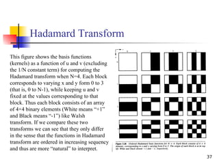
39
Haar Transform
The Haar transform is based on the Haar functions, hk(z), which are defined over the
continuous, closed interval [0,1] for z, and for k=0,1,2,…,N-1, where N=2n
. The first
step in generating the Haar transform is to note that the integer k can be decomposed
uniquely as k=2p
+q-1
where 0≤p≤n-1, q=0 or 1 for p=0, and 1≤q≤2p
for p≠0.
With this background, the Haar functions are defined as
     
   
 























1
,
0
z
for
otherwise
0
2
q
z
2
2
/
1
q
2
2
2
/
1
q
z
2
1
q
2
N
1
z
h
z
h
and
1
,
0
z
for
N
1
z
h
z
h
p
p
2
/
p
p
p
2
/
p
00
k
00
0



40
Haar Transform
 Haar transform matrix for sizes N=2,4,8








1
1
1
1
2
1
Hr2



















2
0
1
1
2
0
1
1
0
2
1
1
0
2
1
1
4
1
Hr4







































2
0
0
0
2
0
1
1
2
0
0
0
2
0
1
1
0
2
0
0
2
0
1
1
0
2
0
0
2
0
1
1
0
0
2
0
0
2
1
1
0
0
2
0
0
2
1
1
0
0
0
2
0
2
1
1
0
0
0
2
0
2
1
1
8
1
Hr8
Can be computed by taking sums and differences.
Fast algorithms by recursively applying Hr2.

43
Slant Transform
 The Slant Transform matrix of order N*N is the recursive expression

44
Slant Transform








1
1
1
1
2
1
S2
 
2
1
2
2
N
1
N
4
N
3
a 







Where I is the identity matrix, and
 
2
1
2
2
N
1
N
4
4
N
b 









45
Slant Transform
Example
Main Image (Gray Level) Slant Transform of Main image
(Slant spectrum)

Karhunen-Loève Transform (KLT)
 a unitary transform with the basis vectors in A being the
“orthonormalized” eigenvectors of Rx

assume real input, write AT
instead of AH

denote the inverse transform matrix as A, AAT
=I

Rx is symmetric for real input, Hermitian for complex input
i.e. Rx
T
=Rx, Rx
H
= Rx

Rx nonnegative definite, i.e. has real non-negative eigen values
 Attributions

Kari Karhunen 1947, Michel Loève 1948

a.k.a Hotelling transform (Harold Hotelling, discrete formulation 1933)

a.k.a. Principle Component Analysis (PCA, estimate Rx from samples)

Decor relation by construction

note: other matrices (unitary or nonunitary) may also de-correlate the transformed sequence [Jain’s example 5.5 and 5.7]
Properties of K-L Transform
 Minimizing MSE under basis restriction
 Basis restriction: Keep only a subset of m transform coefficients and then
perform inverse transform (1 m  N)
 Keep the coefficients w.r.t. the eigenvectors of the first m largest
eigenvalues

discussions about KLT
 The good

Minimum MSE for a “shortened” version
 De-correlating the transform coefficients
 The ugly

Data dependent

Need a good estimate of the second-order statistics

Increased computation complexity
Is there a data-independent transform with similar performance?
data:
linear transform:
estimate Rx:
compute eig Rx:
fast transform:

DCT energy compaction
 DCT is close to KLT for
 DCT is a good replacement for KLT
 Close to optimal for highly correlated data

Not depend on specific data

Fast algorithm available
 highly-correlated first-order stationary Markov source

KL transform for images
 autocorrelation function 1D  2D
 KL basis images are the orthonormalized eigen-functions of R
 rewrite images into vector forms (N2
x1)

solve the eigen problem for N2
xN2
matrix ~ O(N6
)
 if Rx is “separable”
 perform separate KLT on the rows and columns
 transform complexity O(N3
)

KLT on hand-written digits …
1100 digits “6”
16x16 pixels
1100 vectors of size 256x1

Underconstrained Least
Squares
 Problem: if problem very close to singular,
roundoff error can have a huge effect
 Even on “well-determined” values!
 Can detect this:
 Uncertainty proportional to covariance C =
(AT
A)-1
 In other words, unstable if AT
A has small values
 More precisely, care if xT
(AT
A)x is small for any x
 Idea: if part of solution unstable, set answer to 0
 Avoid corrupting good parts of answer

Singular Value
Decomposition (SVD)
 Handy mathematical technique that
has application to many problems
 Given any mn matrix A, algorithm to
find matrices U, V, and W such that
A = UWVT
U is mn and orthonormal
W is nn and diagonal
V is nn and orthonormal

SVD
 Treat as black box: code widely
available
In Matlab: [U,W,V]=svd(A,0)
T
1
0
0
0
0
0
0





















































V
U
A
n
w
w


SVD
 The wi are called the singular values of A
 If A is singular, some of the wi will be 0
 In general rank(A) = number of nonzero wi
 SVD is mostly unique (up to permutation
of singular values, or if some wi are equal)

SVD and Inverses
 Why is SVD so useful?
 Application #1: inverses
 A-1
=(VT
)-1
W-1
U-1
= VW-1
UT
 Using fact that inverse = transpose
for orthogonal matrices
 Since W is diagonal, W-1
also diagonal
with reciprocals of entries of W

SVD and Inverses
 A-1
=(VT
)-1
W-1
U-1
= VW-1
UT
 This fails when some wi are 0
 It’s supposed to fail – singular matrix
 Pseudoinverse: if wi=0, set 1/wi to 0 (!)
 “Closest” matrix to inverse
 Defined for all (even non-square,
singular, etc.) matrices
 Equal to (AT
A)-1
AT
if AT
A invertible

SVD and Least Squares
 Solving Ax=b by least squares
 x=pseudoinverse(A) times b
 Compute pseudoinverse using SVD
 Lets you see if data is singular
 Even if not singular, ratio of max to min
singular values (condition number) tells you
how stable the solution will be
 Set 1/wi to 0 if wi is small (even if not exactly 0)

SVD and Eigenvectors
 Let A=UWVT
, and let xi be ith
column of V
 Consider AT
A xi:
 So elements of W are sqrt(eigenvalues) and
columns of V are eigenvectors of AT
A
 What we wanted for robust least squares fitting!
i
i
i
i
i
i x
w
w
x
x
x
2
2
2
T
2
T
T
T
T
0
0
0
1
0









































V
VW
V
VW
UWV
U
VW
A
A

SVD and Matrix Similarity
 One common definition for the norm of a
matrix is the Frobenius norm:
 Frobenius norm can be computed from
SVD
 So changes to a matrix can be evaluated by
looking at changes to singular values


i j
ij
a
2
F
A


i
i
w
2
F
A

SVD and Matrix Similarity
 Suppose you want to find best rank-k
approximation to A
 Answer: set all but the largest k
singular values to zero
 Can form compact representation by
eliminating columns of U and V
corresponding to zeroed wi

63
Comparison Of Various Transforms

64
Comparison Of Various Transforms

Unit - i-Image Transformations Gonzalez.ppt

More Related Content

Similar to Unit - i-Image Transformations Gonzalez.ppt (20)

More from durgakru (8)

Recently uploaded (20)

Unit - i-Image Transformations Gonzalez.ppt