


![𝐿 𝑊, 𝑏, 𝑊, 𝑏 =
𝑛=1
𝑁
𝑥 𝑛 − 𝑥 𝑥 𝑛
2
If the shape of W is [n,m],
than the shape of 𝑊 is [m,n]
𝑦𝑛
Generally, 𝑊 is not 𝑊 𝑇,
but weight sharing is also possible!
(to reduce the number of parameters)
𝑦1
Autoencoder](https://image.slidesharecdn.com/180208tutorialonvaelabseminar-180720033633/85/Variational-Autoencoder-Tutorial-4-320.jpg)


![input
𝑥
output
𝑓𝜃(𝑥)
data parameter
𝑦𝑓𝜃1 𝑥
𝑝(𝑦| 𝑓𝜃1 𝑥 )𝑚𝑎𝑥𝑖𝑚𝑖𝑧𝑒 𝒑 𝜽 𝒚 𝒙 𝑜𝑟 𝒑 𝒚 𝒇 𝜽 𝒙
𝑚𝑖𝑛𝑖𝑚𝑖𝑧𝑒 − 𝐥𝐨𝐠[𝒑 𝒚 𝒇 𝜽 𝒙 ]
VAE
Explicit density model
assume that 𝑝 𝜃 𝑦 𝑥 follows normal distribution, N(𝑓𝜃 𝑥 , 1)
find 𝑓𝜃 𝑥 that maximize 𝑝 𝜃 𝑦 𝑥 using neural net
Actually, we do this using neural Net!
The output of neural net is parameter of distribution
N(𝑓𝜃 𝑥 , 1) 인 정규분포에서 데이터 y가 나올 확률밀도 값을 얻을 수 있음, 𝒑 𝒚 𝒇 𝜽 𝒙
이를 최대화 하는 방향으로 업데이트!](https://image.slidesharecdn.com/180208tutorialonvaelabseminar-180720033633/85/Variational-Autoencoder-Tutorial-14-320.jpg)
![input
𝑥
output
𝑓𝜃(𝑥)
data parameter
𝑦𝑓𝜃1 𝑥
𝑝(𝑦| 𝑓𝜃1 𝑥 ) <
𝑓𝜃2 𝑥
𝑝(𝑦| 𝑓𝜃2 𝑥 )𝑚𝑎𝑥𝑖𝑚𝑖𝑧𝑒 𝒑 𝜽 𝒚 𝒙 𝑜𝑟 𝒑 𝒚 𝒇 𝜽 𝒙
𝑚𝑖𝑛𝑖𝑚𝑖𝑧𝑒 − 𝐥𝐨𝐠[𝒑 𝒚 𝒇 𝜽 𝒙 ]
VAE
Explicit density model
assume that 𝑝 𝜃 𝑦 𝑥 follows normal distribution, N(𝑓𝜃 𝑥 , 1)
find 𝑓𝜃 𝑥 that maximize 𝑝 𝜃 𝑦 𝑥 using neural net
Actually, we do this using neural Net!
The output of neural net is parameter of distribution](https://image.slidesharecdn.com/180208tutorialonvaelabseminar-180720033633/85/Variational-Autoencoder-Tutorial-15-320.jpg)
![input
𝑥
output
𝑓𝜃(𝑥)
data parameter
𝑦𝑓𝜃1 𝑥 𝑓𝜃2 𝑥 = 𝑓𝜃3 𝑥
𝑚𝑎𝑥𝑖𝑚𝑖𝑧𝑒 𝒑 𝜽 𝒚 𝒙 𝑜𝑟 𝒑 𝒚 𝒇 𝜽 𝒙
𝑚𝑖𝑛𝑖𝑚𝑖𝑧𝑒 − 𝐥𝐨𝐠[𝒑 𝒚 𝒇 𝜽 𝒙 ]
VAE
Explicit density model
assume that 𝑝 𝜃 𝑦 𝑥 follows normal distribution, N(𝑓𝜃 𝑥 , 1)
find 𝑓𝜃 𝑥 that maximize 𝑝 𝜃 𝑦 𝑥 using neural net
Actually, we do this using neural Net!
The output of neural net is parameter of distribution](https://image.slidesharecdn.com/180208tutorialonvaelabseminar-180720033633/85/Variational-Autoencoder-Tutorial-16-320.jpg)


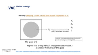
![𝐿 𝑥𝑖 = log 𝑝( 𝑥𝑖)
Let’s use latent variable 𝑧 that follows standard normal distribution N(0, 𝑰)
Let’s assume that 𝒑 𝜽 𝒙 𝒛 𝑜𝑟 𝒑 𝒙 𝒈 𝜽 𝒛 is gaussian with N(𝒈 𝜽 𝒛 , 𝑰) ≈ log 𝑝 𝜃(𝑥𝑖|𝑧)𝑝(𝑧) 𝑑𝑧
= log 𝑝(𝑥𝑖| 𝑔 𝜃 𝑧 )𝑝(𝑧) 𝑑𝑧
= log 𝐸𝑧~𝑝(𝑧)[𝑝 𝑥𝑖 𝑔 𝜃 𝑧 ]
≥ 𝐸𝑧~𝑝(𝑧)[log 𝑝 𝑥𝑖 𝑔 𝜃 𝑧 ]
=
1
𝑀 𝑗=1
𝑀
log 𝑝 𝑥𝑖 𝑔 𝜃 𝑧𝑗 , 𝑧~𝑝(𝑧)
1. 표준정규분포 𝑝(𝑧) 에서 𝑧𝑗 를 셈플링한다.
2. 뉴럴넷을 통해 얻은 값인 𝑔 𝜃 𝑧𝑗 와 실제 𝑥𝑖 가 가까워지도록 gradient descent를 진행한다.
3. 위 과정을 i와 j에 대하여 계속 반복한다.
VAE
Naïve attempt](https://image.slidesharecdn.com/180208tutorialonvaelabseminar-180720033633/85/Variational-Autoencoder-Tutorial-29-320.jpg)


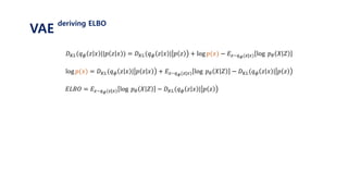
![𝐸𝑧~𝑝(𝑧)[log 𝑝 𝑥𝑖 𝑔 𝜃 𝑧 ]
= 𝑗=1
𝑀
𝑝 𝑥𝑖 𝑔 𝜃 𝑧𝑗 , 𝑧~𝑝(𝑧)
1. 표준정규분포 𝑝(𝑧) 에서 𝑧𝑗 를 셈플링한다.
2. 뉴럴넷을 통해 얻은 값인 𝑔 𝜃 𝑧𝑗 와
실제 𝑥𝑖 가 가까워지도록 gradient descent를 진행한다.
3. 위 과정을 i와 j에 대하여 계속 반복한다.
VAE
variational distribution](https://image.slidesharecdn.com/180208tutorialonvaelabseminar-180720033633/85/Variational-Autoencoder-Tutorial-38-320.jpg)
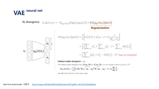
![Let’s use𝐸𝑧~𝑝(𝑧|𝑥 𝑖) log 𝑝 𝑥𝑖 𝑔 𝜃 𝑧 instead of 𝐸𝑧~𝑝(𝑧)
We can now get “differentiating” samples!
However, 𝑝 𝑧 𝑥𝑖 is intractable(cannot calculate)
Therefore, we go variational.
We approximate the posterior 𝑝 𝑧 𝑥𝑖
𝐸𝑧~𝑝(𝑧)[log 𝑝 𝑥𝑖 𝑔 𝜃 𝑧 ]
= 𝑗=1
𝑀
𝑝 𝑥𝑖 𝑔 𝜃 𝑧𝑗 , 𝑧~𝑝(𝑧)
즉, 𝑥𝑖가 주어지면
𝑝 𝑧 𝑥𝑖 에서 𝑧를 𝑠𝑎𝑚𝑝𝑙𝑖𝑛𝑔한 뒤
𝑔 𝜃 𝑧 를 구한 후
𝑥𝑖와 𝑔 𝜃 𝑧 를 비교한다.1. 표준정규분포 𝑝(𝑧) 에서 𝑧𝑗 를 셈플링한다.
2. 뉴럴넷을 통해 얻은 값인 𝑔 𝜃 𝑧𝑗 와
실제 𝑥𝑖 가 가까워지도록 gradient descent를 진행한다.
3. 위 과정을 i와 j에 대하여 계속 반복한다.
VAE
variational distribution](https://image.slidesharecdn.com/180208tutorialonvaelabseminar-180720033633/85/Variational-Autoencoder-Tutorial-39-320.jpg)
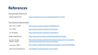
![Since we will never know the posterior 𝑝 𝑧 𝑥𝑖
We approximate it with variational distribution 𝑞 𝜙 𝑧 𝑥𝑖
𝐿 𝑥𝑖 ≅ 𝐸𝑧~𝑝(𝑧)[log 𝑝 𝑥𝑖 𝑔 𝜃 𝑧 ]
𝐿 𝑥𝑖 ≅ 𝐸𝑧~𝑝(𝑧|𝑥 𝑖)[log 𝑝 𝑥𝑖 𝑔 𝜃 𝑧 ]
𝐿 𝑥𝑖 ≅ 𝐸𝑧~𝑞 𝜙(𝑧|𝑥 𝑖)[log 𝑝 𝑥𝑖 𝑔 𝜃 𝑧 ]
With sufficiently good 𝑞 𝜙(𝑧|𝑥𝑖), we will get better gradients
VAE
variational distribution](https://image.slidesharecdn.com/180208tutorialonvaelabseminar-180720033633/85/Variational-Autoencoder-Tutorial-40-320.jpg)


Variational Autoencoder Tutorial
- 1. Tutorial on Variational Autoencoder SKKU Data Mining Lab Hojin Yang
- 3. Autoencoder output is same as input Focus on the middle layer(encoding value) Autoencoder = 자기부호화기 = 자기를 잘 나타내는 부호(encoding 값)를 생성해내는 Neural Net Reducing the dimensionality of data with neural net
- 4. 𝐿 𝑊, 𝑏, 𝑊, 𝑏 = 𝑛=1 𝑁 𝑥 𝑛 − 𝑥 𝑥 𝑛 2 If the shape of W is [n,m], than the shape of 𝑊 is [m,n] 𝑦𝑛 Generally, 𝑊 is not 𝑊 𝑇, but weight sharing is also possible! (to reduce the number of parameters) 𝑦1 Autoencoder
- 6. VAE 식을 어떻게 해석해야 하는가? 뉴럴 넷(Autoencoder)과 어떻게 연결시켜야 하는가? Intro
- 7. VAE The ultimate goal of statistical learning is Learning an underlying distribution from finite data 𝑝(𝑥) 28𝑏𝑦28 mnist data set 𝑥 (28𝑏𝑦28) 0 > 1> 2> … > 6 > … > 9 assume that the frequency of number is motivation
- 8. The ultimate goal of statistical learning is Learning an underlying distribution from finite data 𝑝(𝑥) 28𝑏𝑦28 mnist data set 𝑥 (28𝑏𝑦28) 0 > 1> 2> … > 6 > … > 9 assume that the frequency of number is 𝑥1 The probability density is very high VAE motivation
- 9. The ultimate goal of statistical learning is Learning an underlying distribution from finite data 𝑝(𝑥) 28𝑏𝑦28 mnist data set 𝑥 (28𝑏𝑦28) assume that the frequency of number is 0 > 1> 2> … > 6 > … > 9 The probability density is relatively low 𝑥2 VAE motivation
- 10. The ultimate goal of statistical learning is Learning an underlying distribution from finite data 𝑝(𝑥) 28𝑏𝑦28 mnist data set 𝑥 (28𝑏𝑦28) 0 > 1> 2> … > 6 > … > 9 assume that the frequency of number is 𝑥3 The probability density is almost zero VAE motivation
- 11. If you know 𝑝(𝑥), You can sample some data from 𝑝(𝑥) 𝑝(𝑥) Sampling: Generate 𝑥 ~𝑝(𝑥) Then, how can we learn a distribution from data? Sampling With high probability With extremely low probability 𝑥 (28𝑏𝑦28) VAE motivation
- 12. Set a parametric model 𝑃 𝜃(𝑥), then find 𝜃 Possibly with maximum likelihood or maximum a posteriori For example, if parametric model is Gaussian distribution, then find 𝜇, 𝜎 VAE Explicit density model
- 13. VAE Explicit density model 𝑝(𝑥)는 dataset에 기반해서 고정된 값으로 존재. but 알지 못함(ideal, fixed value) 𝑃 𝜃(𝑥)를 가정하고, dataset에 등장하는 𝑥 값들이 나올 확률을 높이는 식으로 𝑝(𝑥)를 추정 ⇒ 𝑎𝑟𝑔𝑚𝑎𝑥 𝜃 𝑃 𝜃 𝑥
- 14. input 𝑥 output 𝑓𝜃(𝑥) data parameter 𝑦𝑓𝜃1 𝑥 𝑝(𝑦| 𝑓𝜃1 𝑥 )𝑚𝑎𝑥𝑖𝑚𝑖𝑧𝑒 𝒑 𝜽 𝒚 𝒙 𝑜𝑟 𝒑 𝒚 𝒇 𝜽 𝒙 𝑚𝑖𝑛𝑖𝑚𝑖𝑧𝑒 − 𝐥𝐨𝐠[𝒑 𝒚 𝒇 𝜽 𝒙 ] VAE Explicit density model assume that 𝑝 𝜃 𝑦 𝑥 follows normal distribution, N(𝑓𝜃 𝑥 , 1) find 𝑓𝜃 𝑥 that maximize 𝑝 𝜃 𝑦 𝑥 using neural net Actually, we do this using neural Net! The output of neural net is parameter of distribution N(𝑓𝜃 𝑥 , 1) 인 정규분포에서 데이터 y가 나올 확률밀도 값을 얻을 수 있음, 𝒑 𝒚 𝒇 𝜽 𝒙 이를 최대화 하는 방향으로 업데이트!
- 15. input 𝑥 output 𝑓𝜃(𝑥) data parameter 𝑦𝑓𝜃1 𝑥 𝑝(𝑦| 𝑓𝜃1 𝑥 ) < 𝑓𝜃2 𝑥 𝑝(𝑦| 𝑓𝜃2 𝑥 )𝑚𝑎𝑥𝑖𝑚𝑖𝑧𝑒 𝒑 𝜽 𝒚 𝒙 𝑜𝑟 𝒑 𝒚 𝒇 𝜽 𝒙 𝑚𝑖𝑛𝑖𝑚𝑖𝑧𝑒 − 𝐥𝐨𝐠[𝒑 𝒚 𝒇 𝜽 𝒙 ] VAE Explicit density model assume that 𝑝 𝜃 𝑦 𝑥 follows normal distribution, N(𝑓𝜃 𝑥 , 1) find 𝑓𝜃 𝑥 that maximize 𝑝 𝜃 𝑦 𝑥 using neural net Actually, we do this using neural Net! The output of neural net is parameter of distribution
- 16. input 𝑥 output 𝑓𝜃(𝑥) data parameter 𝑦𝑓𝜃1 𝑥 𝑓𝜃2 𝑥 = 𝑓𝜃3 𝑥 𝑚𝑎𝑥𝑖𝑚𝑖𝑧𝑒 𝒑 𝜽 𝒚 𝒙 𝑜𝑟 𝒑 𝒚 𝒇 𝜽 𝒙 𝑚𝑖𝑛𝑖𝑚𝑖𝑧𝑒 − 𝐥𝐨𝐠[𝒑 𝒚 𝒇 𝜽 𝒙 ] VAE Explicit density model assume that 𝑝 𝜃 𝑦 𝑥 follows normal distribution, N(𝑓𝜃 𝑥 , 1) find 𝑓𝜃 𝑥 that maximize 𝑝 𝜃 𝑦 𝑥 using neural net Actually, we do this using neural Net! The output of neural net is parameter of distribution
- 17. VAE Explicit density model https://mega.nz/#!tBo3zAKR!yE6tZ0g-GyUyizDf7uglDk2_ahP-zj5trVZSLW3GAjwSlide from Autoencoder, 이활석
- 18. VAE Explicit density model https://mega.nz/#!tBo3zAKR!yE6tZ0g-GyUyizDf7uglDk2_ahP-zj5trVZSLW3GAjwSlide from Autoencoder, 이활석
- 19. From now, we want to learn 𝑝(𝑥) from data There are two ways to approximate 𝑝(𝑥) using parametric model 𝑥 𝑓𝑟𝑒𝑞 VAE Explicit density model
- 20. From now, we want to learn 𝑝(𝑥) from data There are two ways to approximate 𝑝(𝑥) using parametric model 𝑥 𝑝(𝑥) Set a parametric model 𝑃 𝜃(𝑥), then find 𝜃 𝑃(𝑥)는 gaussian이라 가정하고, MLE를 통해 parameter 𝜃 = 𝜇, 𝜎를 찾자! VAE Explicit density model
- 21. From now, we want to get 𝑝(𝑥) from data There are two ways to approximate 𝑝(𝑥) using parametric model 𝑥 Introduce new latent variable 𝑧~ 𝑃 𝜙(𝑧), And set a parametric model 𝑃 𝜃(𝑥|𝑧), then find 𝜙, 𝜃𝑝(𝑥) VAE Explicit density model
- 22. From now, we want to get 𝑝(𝑥) from data There are two ways to approximate 𝑝(𝑥) using parametric model 𝑥 Introduce new latent variable 𝑧~ 𝑃 𝜙(𝑧), And set a parametric model 𝑃 𝜃(𝑥|𝑧), then find 𝜙, 𝜃 𝑚𝑎𝑥𝑖𝑚𝑖𝑧𝑒 lnP x 𝜙, 𝜃 using E.M algorithm Log likelihood of the dataset is lnP x 𝜙, 𝜃 = 𝑛=1 𝑁 ln 𝑧=0 1 𝑃 𝜙(𝑧) 𝑃 𝜃(𝑥|𝑧) 𝑧~ 𝑃 𝜙(𝑧), 베르누이 분포 따른다고 가정. parameter 𝜙= True 확률 𝑃 𝜃(𝑥|𝑧) , 정규분포 따른다고 가정. Parameter 𝜃 = 𝜇, 𝜎 𝜇, 𝜎 = f(z), g(z) 𝑝(𝑥) VAE Explicit density model
- 23. We are aiming maximize the probability of each x in the dataset, According to: From now, we want to get 𝑝(𝑥) Instead of set parameter on 𝑝 𝜃(𝑥) directly, Let’s use latent variable 𝑧 that follows standard normal distribution N(0, 𝑰) 각도 획 굵기 숫자 … 𝑥 (28𝑏𝑦28) Let’s assume that 𝒑 𝜽 𝒙 𝒛 𝑜𝑟 𝒑 𝒙 𝒈 𝜽 𝒛 is gaussian with N(𝒈 𝜽 𝒛 , 𝑰) 우리가 derive한 p(x) ≈ VAE Explicit density model
- 24. 𝑓 𝑧 𝑝 𝑧 𝑑𝑧 = 𝐸𝑧~𝑝(𝑧) 𝑓(𝑧) 𝑧 ∙ 𝑝 𝑧 𝑑𝑧 = 𝐸𝑧~𝑝(𝑧) 𝑧 VAE preliminary
- 25. 𝑓 𝑧 𝑝 𝑧 𝑑𝑧 = 𝐸𝑧~𝑝(𝑧) 𝑓(𝑧) Monte Carlo approximation 1 𝑁 𝑖=1 𝑁 𝑓(𝑧𝑖), 𝑧𝑖~𝑝(𝑧) 𝑧 ∙ 𝑝 𝑧 𝑑𝑧 = 𝐸𝑧~𝑝(𝑧) 𝑧 1. 𝑝(𝑧)에서 𝑧𝑖를 sampling한 뒤, 𝑓(𝑧𝑖)를 계산. 2. 1을 여러 번 반복한 후 평균 취함. VAE preliminary
- 26. And log is concave VAE preliminary
- 27. Let’s use latent variable 𝑧 that follows standard normal distribution N(0, 𝑰) Let’s assume that 𝒑 𝜽 𝒙 𝒛 𝑜𝑟 𝒑 𝒙 𝒈 𝜽 𝒛 is gaussian with N(𝒈 𝜽 𝒛 , 𝑰) VAE Naïve attempt
- 28. 𝐿 𝑥𝑖 = log 𝑝( 𝑥𝑖) Let’s use latent variable 𝑧 that follows standard normal distribution N(0, 𝑰) Let’s assume that 𝒑 𝜽 𝒙 𝒛 𝑜𝑟 𝒑 𝒙 𝒈 𝜽 𝒛 is gaussian with N(𝒈 𝜽 𝒛 , 𝑰) ≈ log 𝑝 𝜃(𝑥𝑖|𝑧)𝑝(𝑧) 𝑑𝑧 = log 𝑝(𝑥𝑖| 𝑔 𝜃 𝑧 )𝑝(𝑧) 𝑑𝑧 VAE Naïve attempt
- 29. 𝐿 𝑥𝑖 = log 𝑝( 𝑥𝑖) Let’s use latent variable 𝑧 that follows standard normal distribution N(0, 𝑰) Let’s assume that 𝒑 𝜽 𝒙 𝒛 𝑜𝑟 𝒑 𝒙 𝒈 𝜽 𝒛 is gaussian with N(𝒈 𝜽 𝒛 , 𝑰) ≈ log 𝑝 𝜃(𝑥𝑖|𝑧)𝑝(𝑧) 𝑑𝑧 = log 𝑝(𝑥𝑖| 𝑔 𝜃 𝑧 )𝑝(𝑧) 𝑑𝑧 = log 𝐸𝑧~𝑝(𝑧)[𝑝 𝑥𝑖 𝑔 𝜃 𝑧 ] ≥ 𝐸𝑧~𝑝(𝑧)[log 𝑝 𝑥𝑖 𝑔 𝜃 𝑧 ] = 1 𝑀 𝑗=1 𝑀 log 𝑝 𝑥𝑖 𝑔 𝜃 𝑧𝑗 , 𝑧~𝑝(𝑧) 1. 표준정규분포 𝑝(𝑧) 에서 𝑧𝑗 를 셈플링한다. 2. 뉴럴넷을 통해 얻은 값인 𝑔 𝜃 𝑧𝑗 와 실제 𝑥𝑖 가 가까워지도록 gradient descent를 진행한다. 3. 위 과정을 i와 j에 대하여 계속 반복한다. VAE Naïve attempt
- 30. 𝑝(𝑧) 𝑥1 𝑥2 𝑥10… … … 𝑥𝑖 VAE Naïve attempt
- 31. 𝑝(𝑧) 𝑠𝑎𝑚𝑝𝑙𝑖𝑛𝑔 𝑧1,1 = (0.2,0.1) 𝑐𝑎𝑙𝑐𝑢𝑙𝑎𝑡𝑒 𝑑𝑖𝑠𝑡𝑎𝑛𝑐𝑒 𝑥1 𝑥1 𝑥2 𝑥10… … … 𝑥𝑖 VAE Naïve attempt = 1 𝑀 𝑗=1 𝑀 log 𝑝 𝑥𝑖 𝑔 𝜃 𝑧𝑗 , 𝑧~𝑝(𝑧)
- 32. 𝑝(𝑧) 𝑠𝑎𝑚𝑝𝑙𝑖𝑛𝑔 𝑧1,2 = (0.4,1.1) 𝑐𝑎𝑙𝑐𝑢𝑙𝑎𝑡𝑒 𝑑𝑖𝑠𝑡𝑎𝑛𝑐𝑒 𝑥1 𝑥1 𝑥2 𝑥10… … … 𝑥𝑖 VAE Naïve attempt = 1 𝑀 𝑗=1 𝑀 log 𝑝 𝑥𝑖 𝑔 𝜃 𝑧𝑗 , 𝑧~𝑝(𝑧)
- 33. 𝑝(𝑧) 𝑠𝑎𝑚𝑝𝑙𝑖𝑛𝑔 𝑧1,𝑗 = (1.1,0.1) 𝑐𝑎𝑙𝑐𝑢𝑙𝑎𝑡𝑒 𝑑𝑖𝑠𝑡𝑎𝑛𝑐𝑒 𝑥1 𝑥1 𝑥2 𝑥10… … … 𝑥𝑖 VAE Naïve attempt = 1 𝑀 𝑗=1 𝑀 log 𝑝 𝑥𝑖 𝑔 𝜃 𝑧𝑗 , 𝑧~𝑝(𝑧)
- 34. 𝑝(𝑧) 𝑠𝑎𝑚𝑝𝑙𝑖𝑛𝑔 𝑧2,1 = (0.1,0.5) 𝑐𝑎𝑙𝑐𝑢𝑙𝑎𝑡𝑒 𝑑𝑖𝑠𝑡𝑎𝑛𝑐𝑒 𝑥2 𝑥1 𝑥2 𝑥10… … … 𝑥𝑖 VAE Naïve attempt = 1 𝑀 𝑗=1 𝑀 log 𝑝 𝑥𝑖 𝑔 𝜃 𝑧𝑗 , 𝑧~𝑝(𝑧)
- 35. 1 2 34 𝑥1 𝑥2 𝑥10… … … 𝑥𝑖 ≈ VAE Naïve attempt 이상적으로 학습이 되었다면..
- 36. 1 2 34 𝑥1 𝑥2 𝑥10… … … 𝑥𝑖 ≈ VAE Naïve attempt 이상적으로 학습이 되었다면..
- 37. VAE Naïve attempt https://www.slideshare.net/haezoom/variational-autoencoder-understanding-variational-autoencoder-from-various-perspectives slide from VAE 여러 각도에서 이해하기, 윤상웅
- 38. 𝐸𝑧~𝑝(𝑧)[log 𝑝 𝑥𝑖 𝑔 𝜃 𝑧 ] = 𝑗=1 𝑀 𝑝 𝑥𝑖 𝑔 𝜃 𝑧𝑗 , 𝑧~𝑝(𝑧) 1. 표준정규분포 𝑝(𝑧) 에서 𝑧𝑗 를 셈플링한다. 2. 뉴럴넷을 통해 얻은 값인 𝑔 𝜃 𝑧𝑗 와 실제 𝑥𝑖 가 가까워지도록 gradient descent를 진행한다. 3. 위 과정을 i와 j에 대하여 계속 반복한다. VAE variational distribution
- 39. Let’s use𝐸𝑧~𝑝(𝑧|𝑥 𝑖) log 𝑝 𝑥𝑖 𝑔 𝜃 𝑧 instead of 𝐸𝑧~𝑝(𝑧) We can now get “differentiating” samples! However, 𝑝 𝑧 𝑥𝑖 is intractable(cannot calculate) Therefore, we go variational. We approximate the posterior 𝑝 𝑧 𝑥𝑖 𝐸𝑧~𝑝(𝑧)[log 𝑝 𝑥𝑖 𝑔 𝜃 𝑧 ] = 𝑗=1 𝑀 𝑝 𝑥𝑖 𝑔 𝜃 𝑧𝑗 , 𝑧~𝑝(𝑧) 즉, 𝑥𝑖가 주어지면 𝑝 𝑧 𝑥𝑖 에서 𝑧를 𝑠𝑎𝑚𝑝𝑙𝑖𝑛𝑔한 뒤 𝑔 𝜃 𝑧 를 구한 후 𝑥𝑖와 𝑔 𝜃 𝑧 를 비교한다.1. 표준정규분포 𝑝(𝑧) 에서 𝑧𝑗 를 셈플링한다. 2. 뉴럴넷을 통해 얻은 값인 𝑔 𝜃 𝑧𝑗 와 실제 𝑥𝑖 가 가까워지도록 gradient descent를 진행한다. 3. 위 과정을 i와 j에 대하여 계속 반복한다. VAE variational distribution
- 40. Since we will never know the posterior 𝑝 𝑧 𝑥𝑖 We approximate it with variational distribution 𝑞 𝜙 𝑧 𝑥𝑖 𝐿 𝑥𝑖 ≅ 𝐸𝑧~𝑝(𝑧)[log 𝑝 𝑥𝑖 𝑔 𝜃 𝑧 ] 𝐿 𝑥𝑖 ≅ 𝐸𝑧~𝑝(𝑧|𝑥 𝑖)[log 𝑝 𝑥𝑖 𝑔 𝜃 𝑧 ] 𝐿 𝑥𝑖 ≅ 𝐸𝑧~𝑞 𝜙(𝑧|𝑥 𝑖)[log 𝑝 𝑥𝑖 𝑔 𝜃 𝑧 ] With sufficiently good 𝑞 𝜙(𝑧|𝑥𝑖), we will get better gradients VAE variational distribution
- 41. VAE variational distribution https://www.slideshare.net/haezoom/variational-autoencoder-understanding-variational-autoencoder-from-various-perspectives slide from VAE 여러 각도에서 이해하기, 윤상웅
- 42. Now, we have two problems 1. Get 𝑞 𝜙 𝑧 𝑥𝑖 which is similar to 𝑝(𝑧|𝑥𝑖) 2. Maximize 𝐸 𝑧~𝑞 𝜙(𝑧|𝑥 𝑖) log 𝑝 𝑥𝑖 𝑔 𝜃 𝑧 1. How to calculate the distance between 𝑞 𝜙 𝑧 𝑥𝑖 and 𝑝(𝑧|𝑥𝑖)? 2. How much does𝐸 𝑧~𝑞 𝜙(𝑧|𝑥 𝑖) log 𝑝 𝑥𝑖 𝑔 𝜃 𝑧 deviate from the marginal likelihood 𝑝(𝑥𝑖)? Then following questions arise… VAE deriving ELBO
- 43. 𝐷 𝐾𝐿(𝑞 𝜙 𝑧 𝑥 ||𝑝 𝑧 𝑥 ) = 𝑞 𝜙 𝑧 𝑥 log 𝑞 𝜙 𝑧 𝑥 𝑝 𝑧 𝑥 𝑑𝑧 = 𝑞 𝜙 𝑧 𝑥 log 𝑞 𝜙 𝑧 𝑥 ∙ 𝑝(𝑥) 𝑝(𝑧, 𝑥) 𝑑𝑧 = 𝑞 𝜙 𝑧 𝑥 log 𝑞 𝜙 𝑧 𝑥 ∙ 𝑝(𝑥) 𝑝 𝑥 𝑧 ∙ 𝑝(𝑧) 𝑑𝑧 VAE deriving ELBO
- 44. = 𝑞 𝜙 𝑧 𝑥 log 𝑞 𝜙 𝑧 𝑥 ∙ 𝑝(𝑥) 𝑝(𝑧, 𝑥) 𝑑𝑧 = 𝑞 𝜙 𝑧 𝑥 log 𝑞 𝜙 𝑧 𝑥 ∙ 𝑝(𝑥) 𝑝 𝜃 𝑥 𝑧 ∙ 𝑝(𝑧) 𝑑𝑧 = 𝑞 𝜙 𝑧 𝑥 log 𝑞 𝜙 𝑧 𝑥 𝑝(𝑧) 𝑑𝑧 + 𝑞 𝜙 𝑧 𝑥 log 𝑝(𝑥) 𝑑𝑧 − 𝑞 𝜙 𝑧 𝑥 log 𝑝 𝜃(𝑥|𝑧) 𝑑𝑧 = 𝑞 𝜙 𝑧 𝑥 log 𝑞 𝜙 𝑧 𝑥 𝑝(𝑧) 𝑑𝑧 + log 𝑝(𝑥) 𝑞 𝜙 𝑧 𝑥 𝑑𝑧 − 𝑞 𝜙 𝑧 𝑥 log 𝑝 𝜃(𝑥|𝑧) 𝑑𝑧 = 𝑞 𝜙 𝑧 𝑥 log 𝑞 𝜙 𝑧 𝑥 𝑝(𝑧) 𝑑𝑧 + log 𝑝(𝑥) − 𝑞 𝜙 𝑧 𝑥 log 𝑝 𝜃(𝑥|𝑧) 𝑑𝑧 = 𝐷 𝐾𝐿(𝑞 𝜙 𝑧 𝑥 | 𝑝 𝑧 + log 𝑝(𝑥) − 𝐸𝑧~𝑞 𝜙(𝑧|𝑥) log 𝑝 𝜃 𝑋 𝑍 𝐷 𝐾𝐿(𝑞 𝜙 𝑧 𝑥 ||𝑝 𝑧 𝑥 ) = 𝑞 𝜙 𝑧 𝑥 log 𝑞 𝜙 𝑧 𝑥 𝑝 𝑧 𝑥 𝑑𝑧 VAE deriving ELBO
- 45. 𝐷 𝐾𝐿(𝑞 𝜙 𝑧 𝑥 ||𝑝 𝑧 𝑥 ) = 𝐷 𝐾𝐿(𝑞 𝜙 𝑧 𝑥 | 𝑝 𝑧 + log 𝑝(𝑥) − 𝐸𝑧~𝑞 𝜙(𝑧|𝑥) log 𝑝 𝜃 𝑋 𝑍 VAE deriving ELBO
- 46. 𝐷 𝐾𝐿(𝑞 𝜙 𝑧 𝑥 ||𝑝 𝑧 𝑥 ) = 𝐷 𝐾𝐿(𝑞 𝜙 𝑧 𝑥 | 𝑝 𝑧 + log 𝑝(𝑥) − 𝐸𝑧~𝑞 𝜙(𝑧|𝑥) log 𝑝 𝜃 𝑋 𝑍 log 𝑝(𝑥) = 𝐷 𝐾𝐿(𝑞 𝜙 𝑧 𝑥 | 𝑝 𝑧 𝑥 + 𝐸𝑧~𝑞 𝜙(𝑧|𝑥) log 𝑝 𝜃 𝑋 𝑍 − 𝐷 𝐾𝐿(𝑞 𝜙 𝑧 𝑥 | 𝑝 𝑧 𝐸𝐿𝐵𝑂 = 𝐸𝑧~𝑞 𝜙(𝑧|𝑥) log 𝑝 𝜃 𝑋 𝑍 − 𝐷 𝐾𝐿(𝑞 𝜙 𝑧 𝑥 | 𝑝 𝑧 VAE deriving ELBO
- 47. 𝐷 𝐾𝐿(𝑞 𝜙 𝑧 𝑥 ||𝑝 𝑧 𝑥 ) = 𝐷 𝐾𝐿(𝑞 𝜙 𝑧 𝑥 | 𝑝 𝑧 + log 𝑝(𝑥) − 𝐸𝑧~𝑞 𝜙(𝑧|𝑥) log 𝑝 𝜃 𝑋 𝑍 log 𝑝(𝑥) = 𝐷 𝐾𝐿(𝑞 𝜙 𝑧 𝑥 | 𝑝 𝑧 𝑥 + 𝐸𝑧~𝑞 𝜙(𝑧|𝑥) log 𝑝 𝜃 𝑋 𝑍 − 𝐷 𝐾𝐿(𝑞 𝜙 𝑧 𝑥 | 𝑝 𝑧 𝐸𝐿𝐵𝑂 = 𝐸𝑧~𝑞 𝜙(𝑧|𝑥) log 𝑝 𝜃 𝑋 𝑍 − 𝐷 𝐾𝐿(𝑞 𝜙 𝑧 𝑥 | 𝑝 𝑧 log 𝑝(𝑥) Fix! 𝐸𝐿𝐵𝑂 𝐷 𝐾𝐿(𝑞 𝑧 𝑥 | 𝑝 𝑧 𝑥 Remind that we have two problems 1. Get 𝑞 𝜙 𝑧 𝑥 which is similar to 𝑝(𝑧|𝑥) 2. Maximize 𝐸 𝑞 𝜙(𝑧|𝑥) log 𝑝 𝜃 𝑋 𝑍 If we maximize 𝐸𝐿𝐵𝑂 , we can solve both problems! VAE deriving ELBO
- 48. VAE deriving ELBO https://mega.nz/#!tBo3zAKR!yE6tZ0g-GyUyizDf7uglDk2_ahP-zj5trVZSLW3GAjwSlide from Autoencoder, 이활석
- 49. VAE neural net https://mega.nz/#!tBo3zAKR!yE6tZ0g-GyUyizDf7uglDk2_ahP-zj5trVZSLW3GAjwSlide from Autoencoder, 이활석
- 50. X Encoder q(z|x) 𝜇 𝜎 Sample z from q(z|x) decoder p(x|z) 𝜇 = 𝑓(𝑧) VAE neural net 𝑋 − 𝑓 𝑧 2
- 51. VAE neural net
- 52. VAE neural net https://mega.nz/#!tBo3zAKR!yE6tZ0g-GyUyizDf7uglDk2_ahP-zj5trVZSLW3GAjwSlide from Autoencoder, 이활석
- 53. VAE neural net
- 54. VAE neural net
- 55. References 𝑉𝑎𝑟𝑖𝑎𝑡𝑖𝑜𝑛𝑎𝑙 𝐼𝑛𝑓𝑒𝑟𝑒𝑛𝑐𝑒 ratsgo’s blog (Korean) https://ratsgo.github.io/generative%20model/2017/12/19/vi/ 𝑉𝑎𝑟𝑖𝑎𝑡𝑖𝑜𝑛𝑎𝑙 𝐴𝑢𝑡𝑜𝑒𝑛𝑐𝑜𝑑𝑒𝑟 그림 그리는 AI, 이활석 Pr12, 차준범 https://www.youtube.com/watch?v=RYRgX3WD178 https://www.youtube.com/watch?v=KYA-GEhObIs https://www.youtube.com/watch?v=uaaqyVS9-rMLec, Ail Ghodsi ratsgo’s blog (Korean) https://ratsgo.github.io/generative%20model/2018/01/27/VAE/ https://www.slideshare.net/haezoom/variational-autoencoder-understanding- variational-autoencoder-from-various-perspectives VAE 여러 각도에서 이해하기, 윤상웅* https://mega.nz/#!tBo3zAKR!yE6tZ0g-GyUyizDf7uglDk2_ahP-zj5trVZSLW3GAjwAutoencoder, 이활석* http://fbsight.com/t/autoencoder-vae/132132/12Some recommended items