SlideShare a Scribd company logo
Search Algorithms
Prepared by: Afaq Mansoor Khan
BSSE III- Group A
Session 2017-21
IMSciences, Peshawar.
Last Lecture Summary
• Introduction to Data Structures & Algorithms
• One Dimensional Arrays:
• Multi Dimensional Arrays:
▫ Declaration
▫ Initialization
▫ Representation
▫ Operations
▫ Arrays and functions
• Pointers
▫ Declaration, Initialization
▫ Arrays and pointers
Objectives Overview
• Overview of Search Algorithms
• Time and Space Complexity
• Introduction of Linear Searching
• Introduction to Binary Search,
• Comparison of Linear and Binary Search
Algorithms and Complexity
• An algorithm is a well-defined list of steps for solving
a particular problem
• One major challenge of programming is to develop
efficient algorithms for the processing of our data
• The time and space it uses are two major measures
of the efficiency of an algorithm
• The complexity of an algorithm is the function, which
gives the running time and/or space in terms of the
input size
Algorithm Analysis
• Space complexity
▫ How much space is required
• Time complexity
▫ How much time does it take to run the algorithm
Space Complexity
• Space complexity = The amount of memory required
by an algorithm to run to completion
▫ the most often encountered cause is “memory leaks” –
the amount of memory required larger than the
memory available on a given system
• Some algorithms may be more efficient if data
completely loaded into memory
▫ Need to look also at system limitations
▫ e.g. Classify 2GB of text in various categories – can I
afford to load the entire collection?
Space Complexity (cont…)
1. Fixed part: The size required to store certain
data/variables, that is independent of the size of the
problem:
- e.g. name of the data collection
1. Variable part: Space needed by variables, whose size is
dependent on the size of the problem:
- e.g. actual text
- load 2GB of text VS. load 1MB of text
Time Complexity
• Often more important than space complexity
▫ space available tends to be larger and larger
▫ time is still a problem for all of us
• 3-4GHz processors on the market
▫ still …
▫ researchers estimate that the computation of various
transformations for 1 single DNA chain for one single
protein on 1 TerraHZ computer would take about 1 year
to run to completion
• Algorithms running time is an important issue
Time-Space Tradeoff
• Each of our algorithms involves a particular data
structure
• Accordingly, we may not always be able to use the
most efficient algorithm, since the choice of data
structure depends on many things
▫ including the type of data and
▫ frequency with which various data operations are
applied
• Sometimes the choice of data structure involves a
time-space tradeoff:
▫ by increasing the amount of space for storing the data,
one may be able to reduce the time needed for
processing the data, or vice versa
Measuring Efficiency?
• Ways of measuring efficiency:
▫ Run the program and see how long it takes
▫ Run the program and see how much memory it uses
• Lots of variables to control:
▫ What is the input data?
▫ What is the hardware platform?
▫ What is the programming language/compiler?
▫ Just because one program is faster than another right
now, means it will always be faster?
Measuring Efficiency?
• Want to achieve platform-independence
• Use an abstract machine that uses steps of time and
units of memory, instead of seconds or bytes
▫ each elementary operation takes 1 step
▫ each elementary instance occupies 1 unit of memory
Running Time
• Suppose the program includes an if-then statement that
may execute or not:  variable running time
• Typically algorithms are measured by their worst case
Input
1 ms
2 ms
3 ms
4 ms
5 ms
A B C D E F G
worst-case
best-case
}average-case?
A Simple Example
// Input: int A[N], array of N integers
// Output: Sum of all numbers in array A
int Sum(int A[], int N) {
int s=0;
for (int i=0; i< N; i++)
s = s + A[i];
return s;
}
• How should we analyze this?
A Simple Example
• Analysis of Sum
• 1.) Describe the size of the input in terms of one ore
more parameters:
▫ Input to Sum is an array of N ints, so size is N.
• 2.) Then, count how many steps are used for an
input of that size:
▫ A step is an elementary operation such as
+, <, =, A[i]
The Big O Notation
• Used in Computer Science to describe the
performance or complexity of an algorithm.
• Specifically describes the worst-case scenario, and
• can be used to describe the execution time required
or the space used (e.g. in memory or on disk) by an
algorithm
• Characterizes functions according to their growth
rates:
▫ different functions with the same growth rate may be
represented using the same O notation
The Big O Notation
• It is used to describe an algorithm's usage
of computational resources:
▫ the worst case or running time or memory usage of an
algorithm is often expressed as a function of the length
of its input using Big O notation
• Simply, it describes how the algorithm scales
(performs) in the worst case scenario as it is run with
more input
For example
• If we have a sub routine that searches an array item
by item looking for a given element
• The scenario that the Big-O describes is
▫ when the target element is last (or not present at all).
• This particular algorithm is O(N) so the same
algorithm working on an array with 25 elements
should take approximately 5 times longer than an
array with 5 elements
Big O Notation
• This allows algorithm designers to predict the
behavior of their algorithms and to determine which
of multiple algorithms to use, in a way that is
independent of computer architecture or clock rate
• A description of a function in terms of big O notation
usually only provides an upper bound on the growth
rate of the function
Big O Notation
• In typical usage, the formal definition of O notation
is not used directly; rather, the O notation for a
function f(x) is derived by the following simplification
rules:
▫ If f(x) is a sum of several terms, the one with the
largest growth rate is kept, and all others are omitted
▫ If f(x) is a product of several factors, any constants
(terms in the product that do not depend on x) are
omitted
O(1)
• It describes an algorithm that will always execute in
the same time (or space) regardless of the size of the
input data set.
• e.g.
▫ Determining if a number is even or odd
▫ Push and Pop operations for a stack
▫ Insert and Remove operations for a queue
O(N)
• O(N) describes an algorithm whose performance will
grow linearly and in direct proportion to the size of
the input data set.
• Example
▫ Finding the maximum or minimum element in a list, or
sequential search in an unsorted list of n elements
▫ Traversal of a list (a linked list or an array) with n
elements
▫ Example follows as well
O(N2)
• O(N2) represents an algorithm whose performance is
directly proportional to the square of the size of the
input data set.
• Example
▫ Bubble sort
▫ Comparing two 2-dimensional arrays of size n by n
▫ Finding duplicates in an unsorted list of n elements
(implemented with two nested loops)
• This is common with algorithms that involve nested
iterations over the data set.
• Deeper nested iterations will result in O(N3), O(N4)
etc.
O(2N)
• O(2N) denotes an algorithm whose growth will
double with each additional element in the input
data set. The execution time of an O(2N) function will
quickly become very large.
• Big O gives the upper bound for time complexity of
an algorithm. It is usually used in conjunction with
processing data sets (lists) but can be used
elsewhere.
Comparing Functions
Time(steps)
Input (size)
3N = O(N)
0.05 N2 = O(N2)
N = 60
As inputs get larger, any algorithm of a smaller order will
be more efficient than an algorithm of a larger order
Big – O Notation
• Think of f(N) = O(g(N)) as
" f(N) grows at most like g(N)" or
" f grows no faster than g"
(ignoring constant factors, and for large N)
Important:
• Big-O is not a function!
• Never read = as "equals"
• Examples:
5N + 3 = O(N)
37N5 + 7N2 - 2N + 1 = O(N5)
Size Does Matter?
• Common Orders of Growth
O (k) = O (1) Constant Time
O(logbN) = O(log N) Logarithmic Time
O(N) Linear Time
O(N log N)
O(N2) Quadratic Time
O(N3) Cubic Time
--------
O(kN) Exponential Time
IncreasingComplexity
Size Does Matter
• What happens if we double the input size N?
N log2N 5N
Nlog2
N
N2 2N
8 3 40 24 64 256
16 4 80 64 256 65536
32 5 160 160 1024 ~109
64 6 320 384 4096 ~1019
128 7 640 896 16384 ~1038
256 8 1280 2048 65536 ~1076
Standard Analysis Techniques
For a sequence of statements, compute their complexity
Functions individually and add them up
for (j=0; j < N; j++)
for (k =0; k < j; k++)
sum = sum + j*k;
for (l=0; l < N; l++)
sum = sum -l;
printf("sum is now %f", sum);
Total cost is O(N2) + O(N) +O(1) = O(N2)
SUM RULE
• Sequence of Statements
Standard Analysis Techniques
• Digression
When doing Big-O analysis, we sometimes have to compute
a series like:
1 + 2 + 3 + ... + (N-1) + N
What is the complexity of this?
Remember Gauss:
Si = = = O(N2)
i=1
n * (n+1)
2
n2 + n
2
n
Standard Analysis Techniques
• Conditional Statements
What about conditional statements such as
if (condition)
statement1;
else
statement2;
where statement1 runs in O(N) time and
statement2 runs in O(N2) time?
We use "worst case" complexity: among all inputs of
size N, what is the maximum running time?
The analysis for the example above is O(N2)
Searching
• A question you should always ask when selecting a
search algorithm is
• “How fast does the search have to be?”
• The reason is that, in general, the faster the algorithm is,
the more complex it is.
• Bottom line: you don’t always need to use or should use
the fastest algorithm.
• Let’s explore the following search algorithms, keeping
speed in mind.
▫ Sequential (linear) search
▫ Binary search
Searching
• A search algorithm is a method of locating a specific
item of information in a larger collection of data
• Search Algorithms
▫ Computer has organized data into computer memory.
▫ Now we look at various ways of searching for a specific
piece of data or for where to place a specific piece of
data.
▫ Each data item in memory has a unique identification
called its key of the item.
What is Searching
• Finding the location of the record with a given key
value, or finding the locations of some or all records
which satisfy one or more conditions.
• Search algorithms start with a target value and
employ some strategy to visit the elements looking
for a match.
• If target is found, the index of the matching element
becomes the return value.
Linear Search
Linear Search
• In computer science, linear search or sequential search is
a method for finding a particular value in a list, that
consists of checking every one of its elements, one at a
time and in sequence, until the desired one is found
• Linear search is the simplest search algorithm
• Its worst case cost is proportional to the number of
elements in the list; and so is its expected cost, if all list
elements are equally likely to be searched for.
• Therefore, if the list has more than a few elements, other
methods (such as binary search or hashing) will be faster,
but they also impose additional requirements.
Properties of Linear Search
• It is easy to implement.
• It can be applied on random as well as sorted arrays.
• It has more number of comparisons.
• It is better for small inputs not for long inputs.
Linear Search
• Very simple algorithm.
• It uses a loop to sequentially step through an array,
starting with the first element.
• It compares each element with the value being
searched for (key) and stops when that value is
found or the end of the array is reached.
• Can be applied to both sorted and unsorted list
Linear Search - Algorithm
set found to false;
set position to –1;
set index to 0
while (index < number of elements) and (found is false)
if list[index] is equal to search value
found = true
position = index
end if
add 1 to index
end while
return position
Linear Search - Program
Int LinSearch(int [] list, int item, int size) {
int found = 0;
int position = -1;
int index = 0;
while (index < size) && (found == 0) {
if (list[index] == item ) {
found = 1;
position = index;
} // end if
index++;
} // end of while
return position;
} // end of function LinSearch
Linear Search - Example
• Array numlist contains:
• Searching for the the value 11, linear search examines
17, 23, 5, and 11
• Searching for the the value 7, linear search examines
17, 23, 5, 11, 2, 29, and 3
17 23 5 11 2 29 3
Sequential Search of Ordered vs..Unordered List
• Let’s do a comparison.
• If the order was ascending alphabetical on
customer’s last names, how would the search for
John Adams on the ordered list compare with the
search on the unordered list?
▫ Unordered list
 if John Adams was in the list?
 if John Adams was not in the list?
▫ Ordered list
 if John Adams was in the list?
 if John Adams was not in the list?
Ordered Vs. Unordered (Cont…)
• How about George Washington?
▫ Unordered
 if George Washington was in the list?
 If George Washington was not in the list?
▫ Ordered
 if George Washington was in the list?
 If George Washington was not in the list?
• How about James Madison?
Sequential/Linear Search
• If the item we are looking for is the first item, the
search is O(1).
▫ This is the best-case scenario
• If the target item is the last item (item n), the search
takes O(n).
▫ This is the worst-case scenario.
• On average, the item will tend to be near the middle
(n/2) but this can be written (½*n), and as we will see,
we can ignore multiplicative coefficients. Thus, the
average-case is still O(n)
Sequential Search - Analysis
• The following expression gives the average number of
comparisons to find an item in a list size of n:
• It is known that:
• Therefore, the following expression gives the average
number of comparisons made by the sequential search
in the successful case:
Linear Search Tracing
Lets search for the number 3. We start at the beginning and check the first
element in the array. Is it 3?
No, not it. Is it the next element?
Not there either. The next element?
46
Linear Search Tracing
Not there either. Next?
We found it!!! Now you understand the idea of linear searching;
we go through each element, in order, until we find the correct value or
we don’t till the very end.
Linear Search Complexity
• First of all, it is clear that the time required to
execute the algorithm is proportional to the number
of comparisons.
• Also, assuming that each name in the file is equally
likely to be picked, it is intuitively clear that the
average number of comparisons for a file with n
records is equal to n/2;
• that is, the complexity of the linear search algorithm
is given by O(n) for average case
Worst Case Efficiency for Linear Search
1. Get the value of target, n, and the list of n values 1
2. Set index to 1 1
3. Set found to false 1
4. Repeat steps 5-8 until found = true or index > n n
5 if the value of listindex = target then n
6 Output the index 0
7 Set found to true 0
8 else Increment the index by 1 n
9 if not found then 1
10 Print a message that target was not found 0
11 Stop 1
Total 3n+5
Analysis of Sequential Search
• Time efficiency
▫ Best-case : 1 comparison
 target is found immediately
▫ Worst-case: 3n + 5 comparisons
 Target is not found
▫ Average-case: 3n/2+4 comparisons
 Target is found in the middle
• Space efficiency
▫ How much space is used in addition to the
input?
Order of Magnitude
• Worst-case of Linear search:
▫ 3n+5 comparisons
▫ Are these constants accurate? Can we ignore
them?
• Simplification:
▫ ignore the constants, look only at the order of
magnitude
▫ n, 0.5n, 2n, 4n, 3n+5, 2n+100, 0.1n+3 are all
linear
▫ we say that their order of magnitude is n
 3n+5 is order of magnitude n: 3n+5 = (n)
 2n +100 is order of magnitude n: 2n+100=(n)
 0.1n+3 is order of magnitude n: 0.1n+3=(n)
 ….
Linear Search
• The Linear Search algorithm would be impossible in
practice if we were searching through a list
consisting of thousands of names, as in a telephone
book.
• However, if the names are sorted alphabetically, as in
telephone books, then we can use an efficient
algorithm called binary search.
• We may have to use binary search.
Binary Search
The Scenario
• We have a sorted array
• We want to determine if a particular element is in the array
▫ Once found, print or return (index, boolean, etc.)
▫ If not found, indicate the element is not in the collection
7 12 42 59 71 86 104 212
A Better Search Algorithm
• Of course we could use our simpler search and
traverse the array
• But we can use the fact that the array is sorted to
our advantage
• This will allow us to reduce the number of
comparisons
Binary Search
• Requires a sorted array or a binary search tree.
• Cuts the “search space” in half each time.
• Keeps cutting the search space in half until the
target is found or has exhausted the all possible
locations.
The Binary Search Algorithm
calculate middle position
if (first and last have “crossed”) then
“Item not found”
Else if (element at middle = to_find) then
“Item Found”
Else if to_find < element at middle then
Look to the left
else
Look to the right
Binary Search Program
int binarySearch (int list[], int size, int key) {
int first = 0, last , mid, position = -1;
last = size - 1
int found = 0;
while (!found && first <= last) {
middle = (first + last) / 2; /* Calculate mid point */
if (list[mid] == key) { /* If value is found at mid */
found = 1;
position = mid;
}
else if (list[mid] > key) /* If value is in lower half */
last = mid - 1;
else
first = mid + 1; /* If value is in upper half */
} // end while loop
return position;
} // end of function
821 3 4 65 7index 109 11 12 14130
641413 25 33 5143 53value 8472 93 95 97966
 Maintain array of Items
 Store in sorted order
 Use binary search to find Item with key = 33
Binary Search Demo
821 3 4 65 7index 109 11 12 14130
641413 25 33 5143 53value 8472 93 95 97966
rightleft
if Key v is in array, it is
has index between left
and right.
• Maintain array of Items
• Store in sorted order
• Use binary search to find Item with key = 33
821 3 4 65 7index 109 11 12 14130
641413 25 33 5143 53value 8472 93 95 97966
rightleft mid
Compute midpoint and
check if matching Key is in
that position.
 Maintain array of Items
 Store in sorted order
 Use binary search to find Item with key = 33
821 3 4 65 7index 109 11 12 14130
641413 25 33 5143 53value 8472 93 95 97966
lastfirst mid
Since 33 < 53, can reduce
search interval.
 Maintain array of Items
 Store in sorted order
 Use binary search to find Item with key = 33
821 3 4 65 7index 109 11 12 14130
641413 25 33 5143 53value 8472 93 95 97966
lastfirst
Since 33 < 53, can reduce
search interval.
 Maintain array of Items
 Store in sorted order
 Use binary search to find Item with key = 33
821 3 4 65 7index 109 11 12 14130
641413 25 33 5143 53value 8472 93 95 97966
lastfirst mid
Compute midpoint and
check if matching Key is in
that position.
 Maintain array of Items
 Store in sorted order
 Use binary search to find Item with key = 33
821 3 4 65 7index 109 11 12 14130
641413 25 33 5143 53value 8472 93 95 97966
lastfirst mid
Since 33 > 25, can reduce
search interval.
 Maintain array of Items
 Store in sorted order
 Use binary search to find Item with key = 33
821 3 4 65 7index 109 11 12 14130
641413 25 33 5143 53value 8472 93 95 97966
lastfirst
Since 33 > 25, can reduce
search interval.
 Maintain array of Items
 Store in sorted order
 Use binary search to find Item with key = 33
821 3 4 65 7index 109 11 12 14130
641413 25 33 5143 53value 8472 93 95 97966
lastfirst
mid
 Maintain array of Items
 Store in sorted order
 Use binary search to find Item with key = 33
821 3 4 65 7index 109 11 12 14130
641413 25 33 5143 53value 8472 93 95 97966
first
last Compute midpoint and
check if matching Key is in
that position.
 Maintain array of Items
 Store in sorted order
 Use binary search to find Item with key = 33
68
821 3 4 65 7index 109 11 12 14130
641413 25 33 5143 53value 8472 93 95 97966
first
last
Matching Key found.
Return index 4.
 Maintain array of Items
 Store in sorted order
 Use binary search to find Item with key = 33
How Fast is a Binary Search?
• Worst case: 11 items in the list took 4 tries
• How about the worst case for a list with 32 items ?
▫ 1st try - list has 16 items
▫ 2nd try - list has 8 items
▫ 3rd try - list has 4 items
▫ 4th try - list has 2 items
▫ 5th try - list has 1 item
How Fast is a Binary Search?
List has 250 items
1st try - 125 items
2nd try - 63 items
3rd try - 32 items
4th try - 16 items
5th try - 8 items
6th try - 4 items
7th try - 2 items
8th try - 1 item
List has 512 items
1st try - 256 items
2nd try - 128 items
3rd try - 64 items
4th try - 32 items
5th try - 16 items
6th try - 8 items
7th try - 4 items
8th try - 2 items
9th try - 1 item
A Very Fast Algorithm!
• How long (worst case) will it take to find an item in a
list 30,000 items long?
210 = 1024 213 = 8192
211 = 2048 214 = 16384
212 = 4096 215 = 32768
• So, it will take only 15 tries!
• Binary search reduces the work by half at each
comparison
• If array is not sorted  Linear Search
▫ Best Case O(1)
▫ Worst Case O(N)
• If array is sorted  Binary search
▫ Best Case O(1)
▫ Worst Case O(Log2N)
Comparing Search Algorithms
Binary Search
Linear (Sequential) Search
• We know
▫ sequential search is O(n) worst-case
▫ binary search is O(log2 n) worst-case
• Which is better?
• Given n = 1,000,000 items
▫ O(n) = O(1,000,000) /* sequential */
▫ O(log2 n) = O(19) /* binary */
• Clearly binary search is better in worst-case for
large values of n, but there is always trade-offs that
must be considered
▫ Binary search requires the array to be sorted
▫ If the item to be found is near the extremes of the array,
sequential may be faster
Comparing Search Algorithms
Binary Search Tradeoffs
Comparing Sequential and Binary
• The sequential search
starts at the first element
in the list and continues
down the list until either
the item is found or the
entire list has been
searched. If the wanted
item is found, its index is
returned. So it is slow.
• Sequential search is not
efficient because on the
average it needs to search
half a list to find an item.
• A Binary search is much
faster than a sequential
search.
• Binary search works only
on an ordered list.
• Binary search is efficient as
it disregards lower half
after a comparison.
Summary
• Overview of Search Algorithms
• Algorithm Analysis
• Time and Space Complexity
• Big O Notation
• Introduction of Linear Searching
• Introduction to Binary Search,
• Comparison of Linear and Binary Search
References
• https://www.geeksforgeeks.org/searching-
algorithms/
• https://www.studytonight.com/data-
structures/search-algorithms
• https://www.tutorialspoint.com/data_structure
s_algorithms/linear_search_algorithm.htm

More Related Content

What's hot (20)

PPTX
Data Structures - Lecture 9 [Stack & Queue using Linked List]
Muhammad Hammad Waseem
 
PPTX
Asymptotic Notations
Rishabh Soni
 
PPT
Data Structures with C Linked List
Reazul Islam
 
PPTX
Priority queue in DSA
junnubabu
 
PPT
Priority queues
Priyanka Rana
 
PPT
Merge sort
Vidushi Pathak
 
PPTX
Insertion sort algorithm power point presentation
University of Science and Technology Chitttagong
 
PPT
Operating Systems Process Scheduling Algorithms
sathish sak
 
PPT
Hashing
debolina13
 
PPTX
Linear Search Presentation
Markajul Hasnain Alif
 
PPTX
Linked list
Md. Afif Al Mamun
 
PPT
Binary search trees
Dhananjaysinh Jhala
 
PPTX
Analysis of algorithms
iqbalphy1
 
PPTX
Quick sort
Afaq Mansoor Khan
 
PPTX
Quick Sort
Shweta Sahu
 
PPTX
Linked List - Insertion & Deletion
Afaq Mansoor Khan
 
PDF
Algorithms Lecture 4: Sorting Algorithms I
Mohamed Loey
 
PPT
Quick sort Algorithm Discussion And Analysis
SNJ Chaudhary
 
PDF
Singly linked list
Amar Jukuntla
 
Data Structures - Lecture 9 [Stack & Queue using Linked List]
Muhammad Hammad Waseem
 
Asymptotic Notations
Rishabh Soni
 
Data Structures with C Linked List
Reazul Islam
 
Priority queue in DSA
junnubabu
 
Priority queues
Priyanka Rana
 
Merge sort
Vidushi Pathak
 
Insertion sort algorithm power point presentation
University of Science and Technology Chitttagong
 
Operating Systems Process Scheduling Algorithms
sathish sak
 
Hashing
debolina13
 
Linear Search Presentation
Markajul Hasnain Alif
 
Linked list
Md. Afif Al Mamun
 
Binary search trees
Dhananjaysinh Jhala
 
Analysis of algorithms
iqbalphy1
 
Quick sort
Afaq Mansoor Khan
 
Quick Sort
Shweta Sahu
 
Linked List - Insertion & Deletion
Afaq Mansoor Khan
 
Algorithms Lecture 4: Sorting Algorithms I
Mohamed Loey
 
Quick sort Algorithm Discussion And Analysis
SNJ Chaudhary
 
Singly linked list
Amar Jukuntla
 

Similar to Searching Algorithms (20)

PDF
Ch1. Analysis of Algorithms.pdf
zoric99
 
PPTX
Unit ii algorithm
Tribhuvan University
 
PPTX
BCSE202Lkkljkljkbbbnbnghghjghghghghghghghgh
shivapatil54
 
PPTX
Data Structure Algorithm -Algorithm Complexity
zeeshanhaidermazhar7
 
PPTX
02 Introduction to Data Structures & Algorithms.pptx
mettlehenry573
 
PPTX
FALLSEM2022-23_BCSE202L_TH_VL2022230103292_Reference_Material_I_25-07-2022_Fu...
AntareepMajumder
 
PPTX
Algorithms & Complexity Calculation
Akhil Kaushik
 
PPT
Lecture 1 and 2 of Data Structures & Algorithms
haseebanjum2611
 
PDF
Data Structure - Lecture 1 - Introduction.pdf
donotreply20
 
PPTX
Unit 1, ADA.pptx
jinkhatima
 
PDF
1-Algorithm Analysijhjhjhjhjhjhjhjhjhjs.pdf
NGUYNTHNHQUC2
 
PPTX
Algorithm for the DAA agscsnak javausmagagah
RaviPandey598038
 
PDF
DSA
rrupa2
 
PPT
Algorithm analysis
Akshay Dagar
 
PPTX
Design and Analysis of Algorithms.pptx
Syed Zaid Irshad
 
PPT
algorithmAnalysisanddatasteucturesof.ppt
maliozer
 
PPT
Introduction of Analysis of Algorithm , asymptotic notations
namrabsit
 
PPT
Algorithm analysis
sumitbardhan
 
PPTX
2. Introduction to Algorithm.pptx
RahikAhmed1
 
Ch1. Analysis of Algorithms.pdf
zoric99
 
Unit ii algorithm
Tribhuvan University
 
BCSE202Lkkljkljkbbbnbnghghjghghghghghghghgh
shivapatil54
 
Data Structure Algorithm -Algorithm Complexity
zeeshanhaidermazhar7
 
02 Introduction to Data Structures & Algorithms.pptx
mettlehenry573
 
FALLSEM2022-23_BCSE202L_TH_VL2022230103292_Reference_Material_I_25-07-2022_Fu...
AntareepMajumder
 
Algorithms & Complexity Calculation
Akhil Kaushik
 
Lecture 1 and 2 of Data Structures & Algorithms
haseebanjum2611
 
Data Structure - Lecture 1 - Introduction.pdf
donotreply20
 
Unit 1, ADA.pptx
jinkhatima
 
1-Algorithm Analysijhjhjhjhjhjhjhjhjhjs.pdf
NGUYNTHNHQUC2
 
Algorithm for the DAA agscsnak javausmagagah
RaviPandey598038
 
DSA
rrupa2
 
Algorithm analysis
Akshay Dagar
 
Design and Analysis of Algorithms.pptx
Syed Zaid Irshad
 
algorithmAnalysisanddatasteucturesof.ppt
maliozer
 
Introduction of Analysis of Algorithm , asymptotic notations
namrabsit
 
Algorithm analysis
sumitbardhan
 
2. Introduction to Algorithm.pptx
RahikAhmed1
 
Ad

More from Afaq Mansoor Khan (20)

PPTX
Feature Selection - Natural Language Processing
Afaq Mansoor Khan
 
PPTX
WiFi vs LiFi - A Comparison
Afaq Mansoor Khan
 
PPTX
Role of Electronic Media in Pakistan
Afaq Mansoor Khan
 
PPTX
Agile Testing - Approach and Strategies
Afaq Mansoor Khan
 
PPTX
Ethical Hacking - An Overview
Afaq Mansoor Khan
 
PPTX
Software Architecture Design Decisions
Afaq Mansoor Khan
 
PPTX
How to Design an Algorithm
Afaq Mansoor Khan
 
PPTX
Software Quality Qssurance, Scrum and Linkedin
Afaq Mansoor Khan
 
PPTX
.Physics presentation - Asteroids
Afaq Mansoor Khan
 
PPTX
Graph Data Structure
Afaq Mansoor Khan
 
PPTX
AVL Tree Data Structure
Afaq Mansoor Khan
 
PPTX
Binary tree
Afaq Mansoor Khan
 
PPTX
Queue Data Structure
Afaq Mansoor Khan
 
PPTX
Prefix, Infix and Post-fix Notations
Afaq Mansoor Khan
 
PPTX
Stack Data Structure
Afaq Mansoor Khan
 
PPTX
Doubly & Circular Linked Lists
Afaq Mansoor Khan
 
PPTX
Dynamic Memory & Linked Lists
Afaq Mansoor Khan
 
PPTX
Sorting Algorithms
Afaq Mansoor Khan
 
PPTX
Recursion and Sorting Algorithms
Afaq Mansoor Khan
 
PPTX
Introduction to Data Structures & Algorithms
Afaq Mansoor Khan
 
Feature Selection - Natural Language Processing
Afaq Mansoor Khan
 
WiFi vs LiFi - A Comparison
Afaq Mansoor Khan
 
Role of Electronic Media in Pakistan
Afaq Mansoor Khan
 
Agile Testing - Approach and Strategies
Afaq Mansoor Khan
 
Ethical Hacking - An Overview
Afaq Mansoor Khan
 
Software Architecture Design Decisions
Afaq Mansoor Khan
 
How to Design an Algorithm
Afaq Mansoor Khan
 
Software Quality Qssurance, Scrum and Linkedin
Afaq Mansoor Khan
 
.Physics presentation - Asteroids
Afaq Mansoor Khan
 
Graph Data Structure
Afaq Mansoor Khan
 
AVL Tree Data Structure
Afaq Mansoor Khan
 
Binary tree
Afaq Mansoor Khan
 
Queue Data Structure
Afaq Mansoor Khan
 
Prefix, Infix and Post-fix Notations
Afaq Mansoor Khan
 
Stack Data Structure
Afaq Mansoor Khan
 
Doubly & Circular Linked Lists
Afaq Mansoor Khan
 
Dynamic Memory & Linked Lists
Afaq Mansoor Khan
 
Sorting Algorithms
Afaq Mansoor Khan
 
Recursion and Sorting Algorithms
Afaq Mansoor Khan
 
Introduction to Data Structures & Algorithms
Afaq Mansoor Khan
 
Ad

Recently uploaded (20)

PPTX
Customise Your Correlation Table in IBM SPSS Statistics.pptx
Version 1 Analytics
 
PDF
AOMEI Partition Assistant Crack 10.8.2 + WinPE Free Downlaod New Version 2025
bashirkhan333g
 
PPTX
ChiSquare Procedure in IBM SPSS Statistics Version 31.pptx
Version 1 Analytics
 
PPTX
Home Care Tools: Benefits, features and more
Third Rock Techkno
 
PDF
유니티에서 Burst Compiler+ThreadedJobs+SIMD 적용사례
Seongdae Kim
 
PPTX
Tally software_Introduction_Presentation
AditiBansal54083
 
PPTX
Comprehensive Risk Assessment Module for Smarter Risk Management
EHA Soft Solutions
 
PPTX
Coefficient of Variance in IBM SPSS Statistics Version 31.pptx
Version 1 Analytics
 
PPTX
Milwaukee Marketo User Group - Summer Road Trip: Mapping and Personalizing Yo...
bbedford2
 
PPTX
Empowering Asian Contributions: The Rise of Regional User Groups in Open Sour...
Shane Coughlan
 
PDF
AI + DevOps = Smart Automation with devseccops.ai.pdf
Devseccops.ai
 
PPTX
Change Common Properties in IBM SPSS Statistics Version 31.pptx
Version 1 Analytics
 
PDF
MiniTool Power Data Recovery 8.8 With Crack New Latest 2025
bashirkhan333g
 
PDF
SAP Firmaya İade ABAB Kodları - ABAB ile yazılmıl hazır kod örneği
Salih Küçük
 
PPTX
OpenChain @ OSS NA - In From the Cold: Open Source as Part of Mainstream Soft...
Shane Coughlan
 
PDF
Open Chain Q2 Steering Committee Meeting - 2025-06-25
Shane Coughlan
 
PDF
The 5 Reasons for IT Maintenance - Arna Softech
Arna Softech
 
PDF
Automate Cybersecurity Tasks with Python
VICTOR MAESTRE RAMIREZ
 
PDF
Wondershare PDFelement Pro Crack for MacOS New Version Latest 2025
bashirkhan333g
 
PDF
Technical-Careers-Roadmap-in-Software-Market.pdf
Hussein Ali
 
Customise Your Correlation Table in IBM SPSS Statistics.pptx
Version 1 Analytics
 
AOMEI Partition Assistant Crack 10.8.2 + WinPE Free Downlaod New Version 2025
bashirkhan333g
 
ChiSquare Procedure in IBM SPSS Statistics Version 31.pptx
Version 1 Analytics
 
Home Care Tools: Benefits, features and more
Third Rock Techkno
 
유니티에서 Burst Compiler+ThreadedJobs+SIMD 적용사례
Seongdae Kim
 
Tally software_Introduction_Presentation
AditiBansal54083
 
Comprehensive Risk Assessment Module for Smarter Risk Management
EHA Soft Solutions
 
Coefficient of Variance in IBM SPSS Statistics Version 31.pptx
Version 1 Analytics
 
Milwaukee Marketo User Group - Summer Road Trip: Mapping and Personalizing Yo...
bbedford2
 
Empowering Asian Contributions: The Rise of Regional User Groups in Open Sour...
Shane Coughlan
 
AI + DevOps = Smart Automation with devseccops.ai.pdf
Devseccops.ai
 
Change Common Properties in IBM SPSS Statistics Version 31.pptx
Version 1 Analytics
 
MiniTool Power Data Recovery 8.8 With Crack New Latest 2025
bashirkhan333g
 
SAP Firmaya İade ABAB Kodları - ABAB ile yazılmıl hazır kod örneği
Salih Küçük
 
OpenChain @ OSS NA - In From the Cold: Open Source as Part of Mainstream Soft...
Shane Coughlan
 
Open Chain Q2 Steering Committee Meeting - 2025-06-25
Shane Coughlan
 
The 5 Reasons for IT Maintenance - Arna Softech
Arna Softech
 
Automate Cybersecurity Tasks with Python
VICTOR MAESTRE RAMIREZ
 
Wondershare PDFelement Pro Crack for MacOS New Version Latest 2025
bashirkhan333g
 
Technical-Careers-Roadmap-in-Software-Market.pdf
Hussein Ali
 

Searching Algorithms

  • 1. Search Algorithms Prepared by: Afaq Mansoor Khan BSSE III- Group A Session 2017-21 IMSciences, Peshawar.
  • 2. Last Lecture Summary • Introduction to Data Structures & Algorithms • One Dimensional Arrays: • Multi Dimensional Arrays: ▫ Declaration ▫ Initialization ▫ Representation ▫ Operations ▫ Arrays and functions • Pointers ▫ Declaration, Initialization ▫ Arrays and pointers
  • 3. Objectives Overview • Overview of Search Algorithms • Time and Space Complexity • Introduction of Linear Searching • Introduction to Binary Search, • Comparison of Linear and Binary Search
  • 4. Algorithms and Complexity • An algorithm is a well-defined list of steps for solving a particular problem • One major challenge of programming is to develop efficient algorithms for the processing of our data • The time and space it uses are two major measures of the efficiency of an algorithm • The complexity of an algorithm is the function, which gives the running time and/or space in terms of the input size
  • 5. Algorithm Analysis • Space complexity ▫ How much space is required • Time complexity ▫ How much time does it take to run the algorithm
  • 6. Space Complexity • Space complexity = The amount of memory required by an algorithm to run to completion ▫ the most often encountered cause is “memory leaks” – the amount of memory required larger than the memory available on a given system • Some algorithms may be more efficient if data completely loaded into memory ▫ Need to look also at system limitations ▫ e.g. Classify 2GB of text in various categories – can I afford to load the entire collection?
  • 7. Space Complexity (cont…) 1. Fixed part: The size required to store certain data/variables, that is independent of the size of the problem: - e.g. name of the data collection 1. Variable part: Space needed by variables, whose size is dependent on the size of the problem: - e.g. actual text - load 2GB of text VS. load 1MB of text
  • 8. Time Complexity • Often more important than space complexity ▫ space available tends to be larger and larger ▫ time is still a problem for all of us • 3-4GHz processors on the market ▫ still … ▫ researchers estimate that the computation of various transformations for 1 single DNA chain for one single protein on 1 TerraHZ computer would take about 1 year to run to completion • Algorithms running time is an important issue
  • 9. Time-Space Tradeoff • Each of our algorithms involves a particular data structure • Accordingly, we may not always be able to use the most efficient algorithm, since the choice of data structure depends on many things ▫ including the type of data and ▫ frequency with which various data operations are applied • Sometimes the choice of data structure involves a time-space tradeoff: ▫ by increasing the amount of space for storing the data, one may be able to reduce the time needed for processing the data, or vice versa
  • 10. Measuring Efficiency? • Ways of measuring efficiency: ▫ Run the program and see how long it takes ▫ Run the program and see how much memory it uses • Lots of variables to control: ▫ What is the input data? ▫ What is the hardware platform? ▫ What is the programming language/compiler? ▫ Just because one program is faster than another right now, means it will always be faster?
  • 11. Measuring Efficiency? • Want to achieve platform-independence • Use an abstract machine that uses steps of time and units of memory, instead of seconds or bytes ▫ each elementary operation takes 1 step ▫ each elementary instance occupies 1 unit of memory
  • 12. Running Time • Suppose the program includes an if-then statement that may execute or not:  variable running time • Typically algorithms are measured by their worst case Input 1 ms 2 ms 3 ms 4 ms 5 ms A B C D E F G worst-case best-case }average-case?
  • 13. A Simple Example // Input: int A[N], array of N integers // Output: Sum of all numbers in array A int Sum(int A[], int N) { int s=0; for (int i=0; i< N; i++) s = s + A[i]; return s; } • How should we analyze this?
  • 14. A Simple Example • Analysis of Sum • 1.) Describe the size of the input in terms of one ore more parameters: ▫ Input to Sum is an array of N ints, so size is N. • 2.) Then, count how many steps are used for an input of that size: ▫ A step is an elementary operation such as +, <, =, A[i]
  • 15. The Big O Notation • Used in Computer Science to describe the performance or complexity of an algorithm. • Specifically describes the worst-case scenario, and • can be used to describe the execution time required or the space used (e.g. in memory or on disk) by an algorithm • Characterizes functions according to their growth rates: ▫ different functions with the same growth rate may be represented using the same O notation
  • 16. The Big O Notation • It is used to describe an algorithm's usage of computational resources: ▫ the worst case or running time or memory usage of an algorithm is often expressed as a function of the length of its input using Big O notation • Simply, it describes how the algorithm scales (performs) in the worst case scenario as it is run with more input
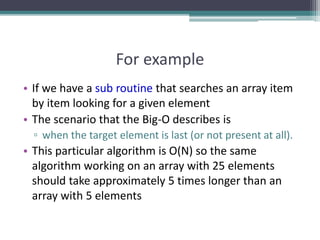
  • 17. For example • If we have a sub routine that searches an array item by item looking for a given element • The scenario that the Big-O describes is ▫ when the target element is last (or not present at all). • This particular algorithm is O(N) so the same algorithm working on an array with 25 elements should take approximately 5 times longer than an array with 5 elements
  • 18. Big O Notation • This allows algorithm designers to predict the behavior of their algorithms and to determine which of multiple algorithms to use, in a way that is independent of computer architecture or clock rate • A description of a function in terms of big O notation usually only provides an upper bound on the growth rate of the function
  • 19. Big O Notation • In typical usage, the formal definition of O notation is not used directly; rather, the O notation for a function f(x) is derived by the following simplification rules: ▫ If f(x) is a sum of several terms, the one with the largest growth rate is kept, and all others are omitted ▫ If f(x) is a product of several factors, any constants (terms in the product that do not depend on x) are omitted
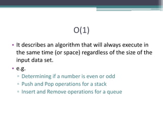
  • 20. O(1) • It describes an algorithm that will always execute in the same time (or space) regardless of the size of the input data set. • e.g. ▫ Determining if a number is even or odd ▫ Push and Pop operations for a stack ▫ Insert and Remove operations for a queue
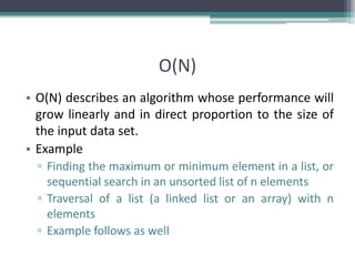
  • 21. O(N) • O(N) describes an algorithm whose performance will grow linearly and in direct proportion to the size of the input data set. • Example ▫ Finding the maximum or minimum element in a list, or sequential search in an unsorted list of n elements ▫ Traversal of a list (a linked list or an array) with n elements ▫ Example follows as well
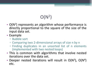
  • 22. O(N2) • O(N2) represents an algorithm whose performance is directly proportional to the square of the size of the input data set. • Example ▫ Bubble sort ▫ Comparing two 2-dimensional arrays of size n by n ▫ Finding duplicates in an unsorted list of n elements (implemented with two nested loops) • This is common with algorithms that involve nested iterations over the data set. • Deeper nested iterations will result in O(N3), O(N4) etc.
  • 23. O(2N) • O(2N) denotes an algorithm whose growth will double with each additional element in the input data set. The execution time of an O(2N) function will quickly become very large. • Big O gives the upper bound for time complexity of an algorithm. It is usually used in conjunction with processing data sets (lists) but can be used elsewhere.
  • 24. Comparing Functions Time(steps) Input (size) 3N = O(N) 0.05 N2 = O(N2) N = 60 As inputs get larger, any algorithm of a smaller order will be more efficient than an algorithm of a larger order
  • 25. Big – O Notation • Think of f(N) = O(g(N)) as " f(N) grows at most like g(N)" or " f grows no faster than g" (ignoring constant factors, and for large N) Important: • Big-O is not a function! • Never read = as "equals" • Examples: 5N + 3 = O(N) 37N5 + 7N2 - 2N + 1 = O(N5)
  • 26. Size Does Matter? • Common Orders of Growth O (k) = O (1) Constant Time O(logbN) = O(log N) Logarithmic Time O(N) Linear Time O(N log N) O(N2) Quadratic Time O(N3) Cubic Time -------- O(kN) Exponential Time IncreasingComplexity
  • 27. Size Does Matter • What happens if we double the input size N? N log2N 5N Nlog2 N N2 2N 8 3 40 24 64 256 16 4 80 64 256 65536 32 5 160 160 1024 ~109 64 6 320 384 4096 ~1019 128 7 640 896 16384 ~1038 256 8 1280 2048 65536 ~1076
  • 28. Standard Analysis Techniques For a sequence of statements, compute their complexity Functions individually and add them up for (j=0; j < N; j++) for (k =0; k < j; k++) sum = sum + j*k; for (l=0; l < N; l++) sum = sum -l; printf("sum is now %f", sum); Total cost is O(N2) + O(N) +O(1) = O(N2) SUM RULE • Sequence of Statements
  • 29. Standard Analysis Techniques • Digression When doing Big-O analysis, we sometimes have to compute a series like: 1 + 2 + 3 + ... + (N-1) + N What is the complexity of this? Remember Gauss: Si = = = O(N2) i=1 n * (n+1) 2 n2 + n 2 n
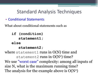
  • 30. Standard Analysis Techniques • Conditional Statements What about conditional statements such as if (condition) statement1; else statement2; where statement1 runs in O(N) time and statement2 runs in O(N2) time? We use "worst case" complexity: among all inputs of size N, what is the maximum running time? The analysis for the example above is O(N2)
  • 31. Searching • A question you should always ask when selecting a search algorithm is • “How fast does the search have to be?” • The reason is that, in general, the faster the algorithm is, the more complex it is. • Bottom line: you don’t always need to use or should use the fastest algorithm. • Let’s explore the following search algorithms, keeping speed in mind. ▫ Sequential (linear) search ▫ Binary search
  • 32. Searching • A search algorithm is a method of locating a specific item of information in a larger collection of data • Search Algorithms ▫ Computer has organized data into computer memory. ▫ Now we look at various ways of searching for a specific piece of data or for where to place a specific piece of data. ▫ Each data item in memory has a unique identification called its key of the item.
  • 33. What is Searching • Finding the location of the record with a given key value, or finding the locations of some or all records which satisfy one or more conditions. • Search algorithms start with a target value and employ some strategy to visit the elements looking for a match. • If target is found, the index of the matching element becomes the return value.
  • 35. Linear Search • In computer science, linear search or sequential search is a method for finding a particular value in a list, that consists of checking every one of its elements, one at a time and in sequence, until the desired one is found • Linear search is the simplest search algorithm • Its worst case cost is proportional to the number of elements in the list; and so is its expected cost, if all list elements are equally likely to be searched for. • Therefore, if the list has more than a few elements, other methods (such as binary search or hashing) will be faster, but they also impose additional requirements.
  • 36. Properties of Linear Search • It is easy to implement. • It can be applied on random as well as sorted arrays. • It has more number of comparisons. • It is better for small inputs not for long inputs.
  • 37. Linear Search • Very simple algorithm. • It uses a loop to sequentially step through an array, starting with the first element. • It compares each element with the value being searched for (key) and stops when that value is found or the end of the array is reached. • Can be applied to both sorted and unsorted list
  • 38. Linear Search - Algorithm set found to false; set position to –1; set index to 0 while (index < number of elements) and (found is false) if list[index] is equal to search value found = true position = index end if add 1 to index end while return position
  • 39. Linear Search - Program Int LinSearch(int [] list, int item, int size) { int found = 0; int position = -1; int index = 0; while (index < size) && (found == 0) { if (list[index] == item ) { found = 1; position = index; } // end if index++; } // end of while return position; } // end of function LinSearch
  • 40. Linear Search - Example • Array numlist contains: • Searching for the the value 11, linear search examines 17, 23, 5, and 11 • Searching for the the value 7, linear search examines 17, 23, 5, 11, 2, 29, and 3 17 23 5 11 2 29 3
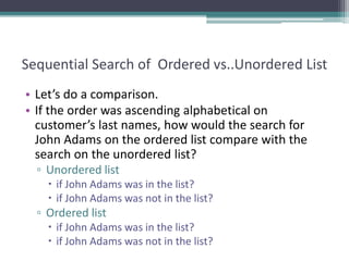
  • 41. Sequential Search of Ordered vs..Unordered List • Let’s do a comparison. • If the order was ascending alphabetical on customer’s last names, how would the search for John Adams on the ordered list compare with the search on the unordered list? ▫ Unordered list  if John Adams was in the list?  if John Adams was not in the list? ▫ Ordered list  if John Adams was in the list?  if John Adams was not in the list?
  • 42. Ordered Vs. Unordered (Cont…) • How about George Washington? ▫ Unordered  if George Washington was in the list?  If George Washington was not in the list? ▫ Ordered  if George Washington was in the list?  If George Washington was not in the list? • How about James Madison?
  • 43. Sequential/Linear Search • If the item we are looking for is the first item, the search is O(1). ▫ This is the best-case scenario • If the target item is the last item (item n), the search takes O(n). ▫ This is the worst-case scenario. • On average, the item will tend to be near the middle (n/2) but this can be written (½*n), and as we will see, we can ignore multiplicative coefficients. Thus, the average-case is still O(n)
  • 44. Sequential Search - Analysis • The following expression gives the average number of comparisons to find an item in a list size of n: • It is known that: • Therefore, the following expression gives the average number of comparisons made by the sequential search in the successful case:
  • 45. Linear Search Tracing Lets search for the number 3. We start at the beginning and check the first element in the array. Is it 3? No, not it. Is it the next element? Not there either. The next element?
  • 46. 46 Linear Search Tracing Not there either. Next? We found it!!! Now you understand the idea of linear searching; we go through each element, in order, until we find the correct value or we don’t till the very end.
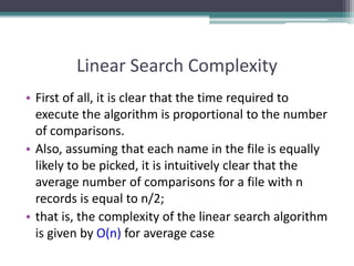
  • 47. Linear Search Complexity • First of all, it is clear that the time required to execute the algorithm is proportional to the number of comparisons. • Also, assuming that each name in the file is equally likely to be picked, it is intuitively clear that the average number of comparisons for a file with n records is equal to n/2; • that is, the complexity of the linear search algorithm is given by O(n) for average case
  • 48. Worst Case Efficiency for Linear Search 1. Get the value of target, n, and the list of n values 1 2. Set index to 1 1 3. Set found to false 1 4. Repeat steps 5-8 until found = true or index > n n 5 if the value of listindex = target then n 6 Output the index 0 7 Set found to true 0 8 else Increment the index by 1 n 9 if not found then 1 10 Print a message that target was not found 0 11 Stop 1 Total 3n+5
  • 49. Analysis of Sequential Search • Time efficiency ▫ Best-case : 1 comparison  target is found immediately ▫ Worst-case: 3n + 5 comparisons  Target is not found ▫ Average-case: 3n/2+4 comparisons  Target is found in the middle • Space efficiency ▫ How much space is used in addition to the input?
  • 50. Order of Magnitude • Worst-case of Linear search: ▫ 3n+5 comparisons ▫ Are these constants accurate? Can we ignore them? • Simplification: ▫ ignore the constants, look only at the order of magnitude ▫ n, 0.5n, 2n, 4n, 3n+5, 2n+100, 0.1n+3 are all linear ▫ we say that their order of magnitude is n  3n+5 is order of magnitude n: 3n+5 = (n)  2n +100 is order of magnitude n: 2n+100=(n)  0.1n+3 is order of magnitude n: 0.1n+3=(n)  ….
  • 51. Linear Search • The Linear Search algorithm would be impossible in practice if we were searching through a list consisting of thousands of names, as in a telephone book. • However, if the names are sorted alphabetically, as in telephone books, then we can use an efficient algorithm called binary search. • We may have to use binary search.
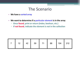
  • 53. The Scenario • We have a sorted array • We want to determine if a particular element is in the array ▫ Once found, print or return (index, boolean, etc.) ▫ If not found, indicate the element is not in the collection 7 12 42 59 71 86 104 212
  • 54. A Better Search Algorithm • Of course we could use our simpler search and traverse the array • But we can use the fact that the array is sorted to our advantage • This will allow us to reduce the number of comparisons
  • 55. Binary Search • Requires a sorted array or a binary search tree. • Cuts the “search space” in half each time. • Keeps cutting the search space in half until the target is found or has exhausted the all possible locations.
  • 56. The Binary Search Algorithm calculate middle position if (first and last have “crossed”) then “Item not found” Else if (element at middle = to_find) then “Item Found” Else if to_find < element at middle then Look to the left else Look to the right
  • 57. Binary Search Program int binarySearch (int list[], int size, int key) { int first = 0, last , mid, position = -1; last = size - 1 int found = 0; while (!found && first <= last) { middle = (first + last) / 2; /* Calculate mid point */ if (list[mid] == key) { /* If value is found at mid */ found = 1; position = mid; } else if (list[mid] > key) /* If value is in lower half */ last = mid - 1; else first = mid + 1; /* If value is in upper half */ } // end while loop return position; } // end of function
  • 58. 821 3 4 65 7index 109 11 12 14130 641413 25 33 5143 53value 8472 93 95 97966  Maintain array of Items  Store in sorted order  Use binary search to find Item with key = 33 Binary Search Demo
  • 59. 821 3 4 65 7index 109 11 12 14130 641413 25 33 5143 53value 8472 93 95 97966 rightleft if Key v is in array, it is has index between left and right. • Maintain array of Items • Store in sorted order • Use binary search to find Item with key = 33
  • 60. 821 3 4 65 7index 109 11 12 14130 641413 25 33 5143 53value 8472 93 95 97966 rightleft mid Compute midpoint and check if matching Key is in that position.  Maintain array of Items  Store in sorted order  Use binary search to find Item with key = 33
  • 61. 821 3 4 65 7index 109 11 12 14130 641413 25 33 5143 53value 8472 93 95 97966 lastfirst mid Since 33 < 53, can reduce search interval.  Maintain array of Items  Store in sorted order  Use binary search to find Item with key = 33
  • 62. 821 3 4 65 7index 109 11 12 14130 641413 25 33 5143 53value 8472 93 95 97966 lastfirst Since 33 < 53, can reduce search interval.  Maintain array of Items  Store in sorted order  Use binary search to find Item with key = 33
  • 63. 821 3 4 65 7index 109 11 12 14130 641413 25 33 5143 53value 8472 93 95 97966 lastfirst mid Compute midpoint and check if matching Key is in that position.  Maintain array of Items  Store in sorted order  Use binary search to find Item with key = 33
  • 64. 821 3 4 65 7index 109 11 12 14130 641413 25 33 5143 53value 8472 93 95 97966 lastfirst mid Since 33 > 25, can reduce search interval.  Maintain array of Items  Store in sorted order  Use binary search to find Item with key = 33
  • 65. 821 3 4 65 7index 109 11 12 14130 641413 25 33 5143 53value 8472 93 95 97966 lastfirst Since 33 > 25, can reduce search interval.  Maintain array of Items  Store in sorted order  Use binary search to find Item with key = 33
  • 66. 821 3 4 65 7index 109 11 12 14130 641413 25 33 5143 53value 8472 93 95 97966 lastfirst mid  Maintain array of Items  Store in sorted order  Use binary search to find Item with key = 33
  • 67. 821 3 4 65 7index 109 11 12 14130 641413 25 33 5143 53value 8472 93 95 97966 first last Compute midpoint and check if matching Key is in that position.  Maintain array of Items  Store in sorted order  Use binary search to find Item with key = 33
  • 68. 68 821 3 4 65 7index 109 11 12 14130 641413 25 33 5143 53value 8472 93 95 97966 first last Matching Key found. Return index 4.  Maintain array of Items  Store in sorted order  Use binary search to find Item with key = 33
  • 69. How Fast is a Binary Search? • Worst case: 11 items in the list took 4 tries • How about the worst case for a list with 32 items ? ▫ 1st try - list has 16 items ▫ 2nd try - list has 8 items ▫ 3rd try - list has 4 items ▫ 4th try - list has 2 items ▫ 5th try - list has 1 item
  • 70. How Fast is a Binary Search? List has 250 items 1st try - 125 items 2nd try - 63 items 3rd try - 32 items 4th try - 16 items 5th try - 8 items 6th try - 4 items 7th try - 2 items 8th try - 1 item List has 512 items 1st try - 256 items 2nd try - 128 items 3rd try - 64 items 4th try - 32 items 5th try - 16 items 6th try - 8 items 7th try - 4 items 8th try - 2 items 9th try - 1 item
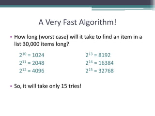
  • 71. A Very Fast Algorithm! • How long (worst case) will it take to find an item in a list 30,000 items long? 210 = 1024 213 = 8192 211 = 2048 214 = 16384 212 = 4096 215 = 32768 • So, it will take only 15 tries!
  • 72. • Binary search reduces the work by half at each comparison • If array is not sorted  Linear Search ▫ Best Case O(1) ▫ Worst Case O(N) • If array is sorted  Binary search ▫ Best Case O(1) ▫ Worst Case O(Log2N)
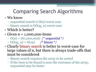
  • 76. • We know ▫ sequential search is O(n) worst-case ▫ binary search is O(log2 n) worst-case • Which is better? • Given n = 1,000,000 items ▫ O(n) = O(1,000,000) /* sequential */ ▫ O(log2 n) = O(19) /* binary */ • Clearly binary search is better in worst-case for large values of n, but there is always trade-offs that must be considered ▫ Binary search requires the array to be sorted ▫ If the item to be found is near the extremes of the array, sequential may be faster Comparing Search Algorithms
  • 78. Comparing Sequential and Binary • The sequential search starts at the first element in the list and continues down the list until either the item is found or the entire list has been searched. If the wanted item is found, its index is returned. So it is slow. • Sequential search is not efficient because on the average it needs to search half a list to find an item. • A Binary search is much faster than a sequential search. • Binary search works only on an ordered list. • Binary search is efficient as it disregards lower half after a comparison.
  • 79. Summary • Overview of Search Algorithms • Algorithm Analysis • Time and Space Complexity • Big O Notation • Introduction of Linear Searching • Introduction to Binary Search, • Comparison of Linear and Binary Search