WSC 2011, advanced tutorial on simulation in Statistics
1 like2,037 views

This document discusses recent advances in simulation methods for statistics. It motivates the use of such methods by explaining how latent variable models can make inference computationally difficult. It introduces Monte Carlo integration and the Metropolis-Hastings algorithm as two important simulation techniques. The document also discusses how Bayesian analysis provides a framework to combine prior information with data, but computing the posterior distribution can be challenging for complex models. Simulation methods are presented as a way to approximate solutions to these computationally difficult statistical problems.


![Simulation methods in Statistics (on recent advances)
Motivation and leading example
Latent variables
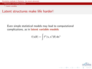
Latent structures make life harder!
Even simple statistical models may lead to computational
complications, as in latent variable models
f(x|θ) = f (x, x |θ) dx
If (x, x ) observed, fine!
If only x observed, trouble!
[mixtures, HMMs, state-space models, &tc]](https://image.slidesharecdn.com/main-111211124711-phpapp02/85/WSC-2011-advanced-tutorial-on-simulation-in-Statistics-6-320.jpg)


![Simulation methods in Statistics (on recent advances)
Motivation and leading example
Inferential methods
Central tool...
Summary in a probability distribution, π(θ|x), called the posterior
distribution
Derived from the joint distribution f(x|θ)π(θ), according to
f(x|θ)π(θ)
π(θ|x) = ,
f(x|θ)π(θ)dθ
[Bayes Theorem]](https://image.slidesharecdn.com/main-111211124711-phpapp02/85/WSC-2011-advanced-tutorial-on-simulation-in-Statistics-20-320.jpg)
![Simulation methods in Statistics (on recent advances)
Motivation and leading example
Inferential methods
Central tool...
Summary in a probability distribution, π(θ|x), called the posterior
distribution
Derived from the joint distribution f(x|θ)π(θ), according to
f(x|θ)π(θ)
π(θ|x) = ,
f(x|θ)π(θ)dθ
[Bayes Theorem]
where
Z(x) = f(x|θ)π(θ)dθ
is the marginal density of X also called the (Bayesian) evidence](https://image.slidesharecdn.com/main-111211124711-phpapp02/85/WSC-2011-advanced-tutorial-on-simulation-in-Statistics-21-320.jpg)


![Simulation methods in Statistics (on recent advances)
Motivation and leading example
Inferential methods
Mixtures again
Observations from
x1 , . . . , xn ∼ f(x|θ) = pϕ(x; µ1 , σ1 ) + (1 − p)ϕ(x; µ2 , σ2 )
Prior
µi |σi ∼ N (ξi , σ2 /ni ),
i σ2 ∼ I G (νi /2, s2 /2),
i i p ∼ Be(α, β)
Posterior
n
π(θ|x1 , . . . , xn ) ∝ pϕ(xj ; µ1 , σ1 ) + (1 − p)ϕ(xj ; µ2 , σ2 ) π(θ)
j=1
n
= ω(kt )π(θ|(kt ))
=0 (kt )
[O(2n )]](https://image.slidesharecdn.com/main-111211124711-phpapp02/85/WSC-2011-advanced-tutorial-on-simulation-in-Statistics-34-320.jpg)
![Simulation methods in Statistics (on recent advances)
Motivation and leading example
Inferential methods
Mixtures again [2]
For a given permutation (kt ), conditional posterior distribution
σ2
π(θ|(kt )) = N ξ1 (kt ), 1
n1 +
×I G ((ν1 + )/2, s1 (kt )/2)
σ22
×N ξ2 (kt ),
n2 + n −
×I G ((ν2 + n − )/2, s2 (kt )/2)
×Be(α + , β + n − )](https://image.slidesharecdn.com/main-111211124711-phpapp02/85/WSC-2011-advanced-tutorial-on-simulation-in-Statistics-35-320.jpg)
![Simulation methods in Statistics (on recent advances)
Motivation and leading example
Inferential methods
Mixtures again [3]
where
1 2
¯
x1 (kt ) = t=1 xkt , ˆ
s1 (kt ) = ¯
t=1 (xkt − x1 (kt )) ,
1 n n 2
¯
x2 (kt ) = n− t= +1 xkt , ˆ
s2 (kt ) = ¯
t= +1 (xkt − x2 (kt ))
and
¯
n1 ξ1 + x1 (kt ) n2 ξ2 + (n − )¯2 (kt )
x
ξ1 (kt ) = , ξ2 (kt ) = ,
n1 + n2 + n −
n1
s1 (kt ) = s2 + s2 (kt ) +
1 ˆ1 (ξ1 − x1 (kt ))2 ,
¯
n1 +
n2 (n − )
s2 (kt ) = s2 + s2 (kt ) +
2 ˆ2 (ξ2 − x2 (kt ))2 ,
¯
n2 + n −
posterior updates of the hyperparameters](https://image.slidesharecdn.com/main-111211124711-phpapp02/85/WSC-2011-advanced-tutorial-on-simulation-in-Statistics-36-320.jpg)
![Simulation methods in Statistics (on recent advances)
Motivation and leading example
Inferential methods
Mixtures again [4]
Bayes estimator of θ:
n
π
δ (x1 , . . . , xn ) = ω(kt )Eπ [θ|x, (kt )]
=0 (kt )
c Too costly: 2n terms](https://image.slidesharecdn.com/main-111211124711-phpapp02/85/WSC-2011-advanced-tutorial-on-simulation-in-Statistics-37-320.jpg)
![Simulation methods in Statistics (on recent advances)
Motivation and leading example
Inferential methods
Mixtures again [4]
Bayes estimator of θ:
n
π
δ (x1 , . . . , xn ) = ω(kt )Eπ [θ|x, (kt )]
=0 (kt )
c Too costly: 2n terms
Unfortunate as the decomposition is meaningfull for clustering
purposes](https://image.slidesharecdn.com/main-111211124711-phpapp02/85/WSC-2011-advanced-tutorial-on-simulation-in-Statistics-38-320.jpg)

![Simulation methods in Statistics (on recent advances)
Monte Carlo Integration
Monte Carlo integration
Monte Carlo integration
Theme:
Generic problem of evaluating the integral
I = Ef [h(X)] = h(x) f(x) dx
X
where X is uni- or multidimensional, f is a closed form, partly
closed form, or implicit density, and h is a function](https://image.slidesharecdn.com/main-111211124711-phpapp02/85/WSC-2011-advanced-tutorial-on-simulation-in-Statistics-40-320.jpg)

![Simulation methods in Statistics (on recent advances)
Monte Carlo Integration
Monte Carlo integration
Monte Carlo integration (2)
Monte Carlo solution
First use a sample (X1 , . . . , Xm ) from the density f to approximate
the integral I by the empirical average
m
1
hm = h(xj )
m
j=1
which converges
hm −→ Ef [h(X)]
by the Strong Law of Large Numbers](https://image.slidesharecdn.com/main-111211124711-phpapp02/85/WSC-2011-advanced-tutorial-on-simulation-in-Statistics-42-320.jpg)
![Simulation methods in Statistics (on recent advances)
Monte Carlo Integration
Monte Carlo integration
Monte Carlo precision
Estimate the variance with
m
1
vm = [h(xj ) − hm ]2 ,
m−1
j=1
and for m large,
hm − Ef [h(X)]
√ ∼ N (0, 1).
vm
Note: This can lead to the construction of a convergence test and
of confidence bounds on the approximation of Ef [h(X)].](https://image.slidesharecdn.com/main-111211124711-phpapp02/85/WSC-2011-advanced-tutorial-on-simulation-in-Statistics-43-320.jpg)


![Simulation methods in Statistics (on recent advances)
Monte Carlo Integration
Importance Sampling
Importance sampling
Paradox
Simulation from f (the true density) is not necessarily optimal
Alternative to direct sampling from f is importance sampling,
based on the alternative representation
f(x)
Ef [h(X)] = h(x) g(x) dx .
X g(x)
which allows us to use other distributions than f](https://image.slidesharecdn.com/main-111211124711-phpapp02/85/WSC-2011-advanced-tutorial-on-simulation-in-Statistics-48-320.jpg)
![Simulation methods in Statistics (on recent advances)
Monte Carlo Integration
Importance Sampling
Importance sampling algorithm
Evaluation of
Ef [h(X)] = h(x) f(x) dx
X
by
1 Generate a sample X1 , . . . , Xn from a distribution g
2 Use the approximation
m
1 f(Xj )
h(Xj )
m g(Xj )
j=1](https://image.slidesharecdn.com/main-111211124711-phpapp02/85/WSC-2011-advanced-tutorial-on-simulation-in-Statistics-49-320.jpg)


![Simulation methods in Statistics (on recent advances)
Monte Carlo Integration
Importance Sampling
Selfnormalised importance sampling
For ratio estimator
n n
δn
h = ωi h(xi ) ωi
i=1 i=1
with Xi ∼ g(y) and Wi such that
E[Wi |Xi = x] = κf(x)/g(x)](https://image.slidesharecdn.com/main-111211124711-phpapp02/85/WSC-2011-advanced-tutorial-on-simulation-in-Statistics-54-320.jpg)
![Simulation methods in Statistics (on recent advances)
Monte Carlo Integration
Importance Sampling
Selfnormalised variance
then
1
var(δn ) ≈
h var(Sn ) − 2Eπ [h] cov(Sn , Sn ) + Eπ [h]2 var(Sn ) .
h h 1 1
n2 κ2
for
n n
Sn =
h Wi h(Xi ) , Sn =
1 Wi
i=1 i=1
Rough approximation
1
varδn ≈
h varπ (h(X)) {1 + varg (W)}
n](https://image.slidesharecdn.com/main-111211124711-phpapp02/85/WSC-2011-advanced-tutorial-on-simulation-in-Statistics-55-320.jpg)


![Simulation methods in Statistics (on recent advances)
Monte Carlo Integration
Bayesian importance sampling
Importance sampling for the Pima Indian dataset
Use of the importance function inspired from the MLE estimate
distribution
β ∼ N(β, Σ)
ˆ ˆ
R Importance sampling code
model1=summary(glm(y~-1+X1,family=binomial(link="probit")))
is1=rmvnorm(Niter,mean=model1$coeff[,1],sigma=2*model1$cov.unscaled)
is2=rmvnorm(Niter,mean=model2$coeff[,1],sigma=2*model2$cov.unscaled)
bfis=mean(exp(probitlpost(is1,y,X1)-dmvlnorm(is1,mean=model1$coeff[,1],
sigma=2*model1$cov.unscaled))) / mean(exp(probitlpost(is2,y,X2)-
dmvlnorm(is2,mean=model2$coeff[,1],sigma=2*model2$cov.unscaled)))](https://image.slidesharecdn.com/main-111211124711-phpapp02/85/WSC-2011-advanced-tutorial-on-simulation-in-Statistics-61-320.jpg)

![Simulation methods in Statistics (on recent advances)
Monte Carlo Integration
Bayesian importance sampling
Bridge sampling
Special case:
If
π1 (θ1 |x) ∝ π1 (θ1 |x)
˜
π2 (θ2 |x) ∝ π2 (θ2 |x)
˜
live on the same space (Θ1 = Θ2 ), then
n
1 π1 (θi |x)
˜
B12 ≈ θi ∼ π2 (θ|x)
n π2 (θi |x)
˜
i=1
[Gelman & Meng, 1998; Chen, Shao & Ibrahim, 2000]](https://image.slidesharecdn.com/main-111211124711-phpapp02/85/WSC-2011-advanced-tutorial-on-simulation-in-Statistics-63-320.jpg)


![Simulation methods in Statistics (on recent advances)
Monte Carlo Integration
Bayesian importance sampling
Illustration for the Pima Indian dataset
Use of the MLE induced conditional of β3 given (β1 , β2 ) as a
pseudo-posterior and mixture of both MLE approximations on β3
in bridge sampling estimate
R bridge sampling code
cova=model2$cov.unscaled
expecta=model2$coeff[,1]
covw=cova[3,3]-t(cova[1:2,3])%*%ginv(cova[1:2,1:2])%*%cova[1:2,3]
probit1=hmprobit(Niter,y,X1)
probit2=hmprobit(Niter,y,X2)
pseudo=rnorm(Niter,meanw(probit1),sqrt(covw))
probit1p=cbind(probit1,pseudo)
bfbs=mean(exp(probitlpost(probit2[,1:2],y,X1)+dnorm(probit2[,3],meanw(probit2[,1:2]),
sqrt(covw),log=T))/ (dmvnorm(probit2,expecta,cova)+dnorm(probit2[,3],expecta[3],
cova[3,3])))/ mean(exp(probitlpost(probit1p,y,X2))/(dmvnorm(probit1p,expecta,cova)+
dnorm(pseudo,expecta[3],cova[3,3])))](https://image.slidesharecdn.com/main-111211124711-phpapp02/85/WSC-2011-advanced-tutorial-on-simulation-in-Statistics-67-320.jpg)

![Simulation methods in Statistics (on recent advances)
Monte Carlo Integration
Bayesian importance sampling
The original harmonic mean estimator
When θki ∼ πk (θ|x),
T
1 1
T L(θkt |x)
t=1
is an unbiased estimator of 1/mk (x)
[Newton & Raftery, 1994]](https://image.slidesharecdn.com/main-111211124711-phpapp02/85/WSC-2011-advanced-tutorial-on-simulation-in-Statistics-69-320.jpg)
![Simulation methods in Statistics (on recent advances)
Monte Carlo Integration
Bayesian importance sampling
The original harmonic mean estimator
When θki ∼ πk (θ|x),
T
1 1
T L(θkt |x)
t=1
is an unbiased estimator of 1/mk (x)
[Newton & Raftery, 1994]
Highly dangerous: Most often leads to an infinite variance!!!](https://image.slidesharecdn.com/main-111211124711-phpapp02/85/WSC-2011-advanced-tutorial-on-simulation-in-Statistics-70-320.jpg)

![Simulation methods in Statistics (on recent advances)
Monte Carlo Integration
Bayesian importance sampling
“The Worst Monte Carlo Method Ever”
“The good news is that the Law of Large Numbers guarantees that
this estimator is consistent ie, it will very likely be very close to the
correct answer if you use a sufficiently large number of points from
the posterior distribution.
The bad news is that the number of points required for this
estimator to get close to the right answer will often be greater
than the number of atoms in the observable universe. The even
worse news is that it’s easy for people to not realize this, and to
na¨ıvely accept estimates that are nowhere close to the correct
value of the marginal likelihood.”
[Radford Neal’s blog, Aug. 23, 2008]](https://image.slidesharecdn.com/main-111211124711-phpapp02/85/WSC-2011-advanced-tutorial-on-simulation-in-Statistics-72-320.jpg)
![Simulation methods in Statistics (on recent advances)
Monte Carlo Integration
Bayesian importance sampling
Approximating Zk from a posterior sample
Use of the [harmonic mean] identity
ϕ(θk ) ϕ(θk ) πk (θk )Lk (θk ) 1
Eπk x = dθk =
πk (θk )Lk (θk ) πk (θk )Lk (θk ) Zk Zk
no matter what the proposal ϕ(·) is.
[Gelfand & Dey, 1994; Bartolucci et al., 2006]](https://image.slidesharecdn.com/main-111211124711-phpapp02/85/WSC-2011-advanced-tutorial-on-simulation-in-Statistics-73-320.jpg)
![Simulation methods in Statistics (on recent advances)
Monte Carlo Integration
Bayesian importance sampling
Approximating Zk from a posterior sample
Use of the [harmonic mean] identity
ϕ(θk ) ϕ(θk ) πk (θk )Lk (θk ) 1
Eπk x = dθk =
πk (θk )Lk (θk ) πk (θk )Lk (θk ) Zk Zk
no matter what the proposal ϕ(·) is.
[Gelfand & Dey, 1994; Bartolucci et al., 2006]
Direct exploitation of the MCMC output](https://image.slidesharecdn.com/main-111211124711-phpapp02/85/WSC-2011-advanced-tutorial-on-simulation-in-Statistics-74-320.jpg)


![Simulation methods in Statistics (on recent advances)
Monte Carlo Integration
Bayesian importance sampling
Chib’s representation
Direct application of Bayes’ theorem: given x ∼ fk (x|θk ) and
θk ∼ πk (θk ),
fk (x|θk ) πk (θk )
mk (x) =
πk (θk |x)
[Bayes Theorem]](https://image.slidesharecdn.com/main-111211124711-phpapp02/85/WSC-2011-advanced-tutorial-on-simulation-in-Statistics-79-320.jpg)
![Simulation methods in Statistics (on recent advances)
Monte Carlo Integration
Bayesian importance sampling
Chib’s representation
Direct application of Bayes’ theorem: given x ∼ fk (x|θk ) and
θk ∼ πk (θk ),
fk (x|θk ) πk (θk )
mk (x) =
πk (θk |x)
[Bayes Theorem]
Use of an approximation to the posterior
fk (x|θ∗ ) πk (θ∗ )
k k
mk (x) = .
πk (θ∗ |x)
ˆ k](https://image.slidesharecdn.com/main-111211124711-phpapp02/85/WSC-2011-advanced-tutorial-on-simulation-in-Statistics-80-320.jpg)

![Simulation methods in Statistics (on recent advances)
Monte Carlo Integration
Bayesian importance sampling
Case of the probit model
For the completion by z,
1
ˆ
π(θ|x) = π(θ|x, z(t) )
T t
is a simple average of normal densities
R Bridge sampling code
gibbs1=gibbsprobit(Niter,y,X1)
gibbs2=gibbsprobit(Niter,y,X2)
bfchi=mean(exp(dmvlnorm(t(t(gibbs2$mu)-model2$coeff[,1]),mean=rep(0,3),
sigma=gibbs2$Sigma2)-probitlpost(model2$coeff[,1],y,X2)))/
mean(exp(dmvlnorm(t(t(gibbs1$mu)-model1$coeff[,1]),mean=rep(0,2),
sigma=gibbs1$Sigma2)-probitlpost(model1$coeff[,1],y,X1)))](https://image.slidesharecdn.com/main-111211124711-phpapp02/85/WSC-2011-advanced-tutorial-on-simulation-in-Statistics-83-320.jpg)


![Simulation methods in Statistics (on recent advances)
The Metropolis-Hastings Algorithm
Monte Carlo Methods based on Markov Chains
Running Monte Carlo via Markov Chains
Epiphany! It is not necessary to use a sample from the distribution
f to approximate the integral
I= h(x)f(x)dx ,
Principle: Obtain X1 , . . . , Xn ∼ f (approx) without directly
simulating from f, using an ergodic Markov chain with stationary
distribution f
[Metropolis et al., 1953]](https://image.slidesharecdn.com/main-111211124711-phpapp02/85/WSC-2011-advanced-tutorial-on-simulation-in-Statistics-87-320.jpg)


![Simulation methods in Statistics (on recent advances)
The Metropolis-Hastings Algorithm
The random walk Metropolis-Hastings algorithm
Acceptance rate
A high acceptance rate is not indication of efficiency since the
random walk may be moving “too slowly” on the target surface
If average acceptance rate low, the proposed values f(yt ) tend to
be small wrt f(x(t) ), i.e. the random walk [not the algorithm!]
moves quickly on the target surface often reaching its boundaries](https://image.slidesharecdn.com/main-111211124711-phpapp02/85/WSC-2011-advanced-tutorial-on-simulation-in-Statistics-101-320.jpg)
![Simulation methods in Statistics (on recent advances)
The Metropolis-Hastings Algorithm
The random walk Metropolis-Hastings algorithm
Rule of thumb
In small dimensions, aim at an average acceptance rate of 50%. In
large dimensions, at an average acceptance rate of 25%.
[Gelman,Gilks and Roberts, 1995]](https://image.slidesharecdn.com/main-111211124711-phpapp02/85/WSC-2011-advanced-tutorial-on-simulation-in-Statistics-102-320.jpg)


![Simulation methods in Statistics (on recent advances)
The Metropolis-Hastings Algorithm
Adaptive MCMC
No free lunch!!
MCMC algorithm trained on-line usually invalid:
using the whole past of the “chain” implies that this is not a
Markov chain any longer!
This means standard Markov chain (ergodic) theory does not apply
[Meyn & Tweedie, 1994]](https://image.slidesharecdn.com/main-111211124711-phpapp02/85/WSC-2011-advanced-tutorial-on-simulation-in-Statistics-108-320.jpg)


![Simulation methods in Statistics (on recent advances)
The Metropolis-Hastings Algorithm
Adaptive MCMC
Simply forget about it!
Warning:
One should not constantly adapt the proposal on past
performances
Either adaptation ceases after a period of burnin...
or the adaptive scheme must be theoretically assessed on its own
right.
[Haario & Saaksman, 1999;Andrieu & Robert, 2001]](https://image.slidesharecdn.com/main-111211124711-phpapp02/85/WSC-2011-advanced-tutorial-on-simulation-in-Statistics-114-320.jpg)
![Simulation methods in Statistics (on recent advances)
The Metropolis-Hastings Algorithm
Adaptive MCMC
Diminishing adaptation
Adaptivity of cyberparameter γt has to be gradually tuned down
to recover ergodicity
[Roberts & Rosenthal, 2007]](https://image.slidesharecdn.com/main-111211124711-phpapp02/85/WSC-2011-advanced-tutorial-on-simulation-in-Statistics-115-320.jpg)
![Simulation methods in Statistics (on recent advances)
The Metropolis-Hastings Algorithm
Adaptive MCMC
Diminishing adaptation
Adaptivity of cyberparameter γt has to be gradually tuned down
to recover ergodicity
[Roberts & Rosenthal, 2007]
Sufficient conditions:
1 total variation distance between two consecutive kernels must
uniformly decrease to zero
[diminishing adaptation]
lim sup Kγt (x, ·) − Kγt+1 (x, ·) TV =0
t→∞ x
2 times to stationary remains bounded for any fixed γt
[containment]](https://image.slidesharecdn.com/main-111211124711-phpapp02/85/WSC-2011-advanced-tutorial-on-simulation-in-Statistics-116-320.jpg)
![Simulation methods in Statistics (on recent advances)
The Metropolis-Hastings Algorithm
Adaptive MCMC
Diminishing adaptation
Adaptivity of cyberparameter γt has to be gradually tuned down
to recover ergodicity
[Roberts & Rosenthal, 2007]
Sufficient conditions:
1 total variation distance between two consecutive kernels must
uniformly decrease to zero
[diminishing adaptation]
lim sup Kγt (x, ·) − Kγt+1 (x, ·) TV =0
t→∞ x
2 times to stationary remains bounded for any fixed γt
[containment]
Works for random walk proposal that relies on the
empirical variance of the sample modulo a ridge-like stabilizing factor
[Haario, Sacksman & Tamminen, 1999]](https://image.slidesharecdn.com/main-111211124711-phpapp02/85/WSC-2011-advanced-tutorial-on-simulation-in-Statistics-117-320.jpg)
![Simulation methods in Statistics (on recent advances)
The Metropolis-Hastings Algorithm
Adaptive MCMC
Diminishing adaptation
Adaptivity of cyberparameter γt has to be gradually tuned down
to recover ergodicity
[Roberts & Rosenthal, 2007]
Sufficient conditions:
1 total variation distance between two consecutive kernels must
uniformly decrease to zero
[diminishing adaptation]
lim sup Kγt (x, ·) − Kγt+1 (x, ·) TV =0
t→∞ x
2 times to stationary remains bounded for any fixed γt
[containment]
Tune the scale in each direction toward an optimal acceptance rate
of 0.44.
[Roberts & Rosenthal,2006]](https://image.slidesharecdn.com/main-111211124711-phpapp02/85/WSC-2011-advanced-tutorial-on-simulation-in-Statistics-118-320.jpg)
![Simulation methods in Statistics (on recent advances)
The Metropolis-Hastings Algorithm
Adaptive MCMC
Diminishing adaptation
Adaptivity of cyberparameter γt has to be gradually tuned down
to recover ergodicity
[Roberts & Rosenthal, 2007]
Sufficient conditions:
1 total variation distance between two consecutive kernels must
uniformly decrease to zero
[diminishing adaptation]
lim sup Kγt (x, ·) − Kγt+1 (x, ·) TV =0
t→∞ x
2 times to stationary remains bounded for any fixed γt
[containment]
Packages amcmc and grapham](https://image.slidesharecdn.com/main-111211124711-phpapp02/85/WSC-2011-advanced-tutorial-on-simulation-in-Statistics-119-320.jpg)

![Simulation methods in Statistics (on recent advances)
Approximate Bayesian computation
ABC basics
Untractable likelihoods
There are cases when the likelihood function f(y|θ) is unavailable
and when the completion step
f(y|θ) = f(y, z|θ) dz
Z
is impossible or too costly because of the dimension of z
c MCMC cannot be implemented!
[Robert & Casella, 2004]](https://image.slidesharecdn.com/main-111211124711-phpapp02/85/WSC-2011-advanced-tutorial-on-simulation-in-Statistics-121-320.jpg)


![Simulation methods in Statistics (on recent advances)
Approximate Bayesian computation
ABC basics
Illustrations
Example
Inference on CMB: in cosmology, study of the Cosmic Microwave
Background via likelihoods immensely slow to computate (e.g
WMAP, Plank), because of numerically costly spectral transforms
[Data is a Fortran program]
[Kilbinger et al., 2010, MNRAS]](https://image.slidesharecdn.com/main-111211124711-phpapp02/85/WSC-2011-advanced-tutorial-on-simulation-in-Statistics-124-320.jpg)
![Simulation methods in Statistics (on recent advances)
Approximate Bayesian computation
ABC basics
Illustrations
Example
Coalescence tree: in population
genetics, reconstitution of a common
ancestor from a sample of genes via
a phylogenetic tree that is close to
impossible to integrate out
[100 processor days with 4
parameters]
[Cornuet et al., 2009, Bioinformatics]](https://image.slidesharecdn.com/main-111211124711-phpapp02/85/WSC-2011-advanced-tutorial-on-simulation-in-Statistics-125-320.jpg)

![Simulation methods in Statistics (on recent advances)
Approximate Bayesian computation
ABC basics
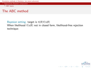
The ABC method
Bayesian setting: target is π(θ)f(x|θ)
When likelihood f(x|θ) not in closed form, likelihood-free rejection
technique:
ABC algorithm
For an observation y ∼ f(y|θ), under the prior π(θ), keep jointly
simulating
θ ∼ π(θ) , z ∼ f(z|θ ) ,
until the auxiliary variable z is equal to the observed value, z = y.
[Tavar´ et al., 1997]
e](https://image.slidesharecdn.com/main-111211124711-phpapp02/85/WSC-2011-advanced-tutorial-on-simulation-in-Statistics-128-320.jpg)
![Simulation methods in Statistics (on recent advances)
Approximate Bayesian computation
ABC basics
Why does it work?!
The proof is trivial:
f(θi ) ∝ π(θi )f(z|θi )Iy (z)
z∈D
∝ π(θi )f(y|θi )
= π(θi |y) .
[Accept–Reject 101]](https://image.slidesharecdn.com/main-111211124711-phpapp02/85/WSC-2011-advanced-tutorial-on-simulation-in-Statistics-129-320.jpg)
![Simulation methods in Statistics (on recent advances)
Approximate Bayesian computation
ABC basics
Earlier occurrence
‘Bayesian statistics and Monte Carlo methods are ideally
suited to the task of passing many models over one
dataset’
[Don Rubin, Annals of Statistics, 1984]
Note Rubin (1984) does not promote this algorithm for
likelihood-free simulation but frequentist intuition on posterior
distributions: parameters from posteriors are more likely to be
those that could have generated the data.](https://image.slidesharecdn.com/main-111211124711-phpapp02/85/WSC-2011-advanced-tutorial-on-simulation-in-Statistics-130-320.jpg)


![Simulation methods in Statistics (on recent advances)
Approximate Bayesian computation
ABC basics
ABC advances
Simulating from the prior is often poor in efficiency
Either modify the proposal distribution on θ to increase the density
of x’s within the vicinity of y...
[Marjoram et al, 2003; Bortot et al., 2007, Sisson et al., 2007]](https://image.slidesharecdn.com/main-111211124711-phpapp02/85/WSC-2011-advanced-tutorial-on-simulation-in-Statistics-144-320.jpg)
![Simulation methods in Statistics (on recent advances)
Approximate Bayesian computation
ABC basics
ABC advances
Simulating from the prior is often poor in efficiency
Either modify the proposal distribution on θ to increase the density
of x’s within the vicinity of y...
[Marjoram et al, 2003; Bortot et al., 2007, Sisson et al., 2007]
...or by viewing the problem as a conditional density estimation
and by developing techniques to allow for larger
[Beaumont et al., 2002]](https://image.slidesharecdn.com/main-111211124711-phpapp02/85/WSC-2011-advanced-tutorial-on-simulation-in-Statistics-145-320.jpg)
![Simulation methods in Statistics (on recent advances)
Approximate Bayesian computation
ABC basics
ABC advances
Simulating from the prior is often poor in efficiency
Either modify the proposal distribution on θ to increase the density
of x’s within the vicinity of y...
[Marjoram et al, 2003; Bortot et al., 2007, Sisson et al., 2007]
...or by viewing the problem as a conditional density estimation
and by developing techniques to allow for larger
[Beaumont et al., 2002]
.....or even by including in the inferential framework [ABCµ ]
[Ratmann et al., 2009]](https://image.slidesharecdn.com/main-111211124711-phpapp02/85/WSC-2011-advanced-tutorial-on-simulation-in-Statistics-146-320.jpg)
![Simulation methods in Statistics (on recent advances)
Approximate Bayesian computation
Alphabet soup
ABC-NP
Better usage of [prior] simulations by
adjustement: instead of throwing away
θ such that ρ(η(z), η(y)) > , replace
θs with locally regressed
θ∗ = θ − {η(z) − η(y)}T β
ˆ
[Csill´ry et al., TEE, 2010]
e
ˆ
where β is obtained by [NP] weighted least square regression on
(η(z) − η(y)) with weights
Kδ {ρ(η(z), η(y))}
[Beaumont et al., 2002, Genetics]](https://image.slidesharecdn.com/main-111211124711-phpapp02/85/WSC-2011-advanced-tutorial-on-simulation-in-Statistics-147-320.jpg)

![Simulation methods in Statistics (on recent advances)
Approximate Bayesian computation
Alphabet soup
ABC-MCMC
Markov chain (θ(t) ) created via the transition function
θ ∼ Kω (θ |θ(t) ) if x ∼ f(x|θ ) is such that x = y
π(θ )Kω (t) |θ )
θ(t+1)
= and u ∼ U(0, 1) π(θ(t) )K (θ |θ(t) ) ,
(t) ω (θ
θ otherwise,
has the posterior π(θ|y) as stationary distribution
[Marjoram et al, 2003]](https://image.slidesharecdn.com/main-111211124711-phpapp02/85/WSC-2011-advanced-tutorial-on-simulation-in-Statistics-149-320.jpg)
![Simulation methods in Statistics (on recent advances)
Approximate Bayesian computation
Alphabet soup
ABC-MCMC (2)
Algorithm 2 Likelihood-free MCMC sampler
Use Algorithm 1 to get (θ(0) , z(0) )
for t = 1 to N do
Generate θ from Kω ·|θ(t−1) ,
Generate z from the likelihood f(·|θ ),
Generate u from U[0,1] ,
π(θ )Kω (θ(t−1) |θ )
if u I
π(θ(t−1) Kω (θ |θ(t−1) ) A ,y (z ) then
set (θ(t) , z(t) ) = (θ , z )
else
(θ(t) , z(t) )) = (θ(t−1) , z(t−1) ),
end if
end for](https://image.slidesharecdn.com/main-111211124711-phpapp02/85/WSC-2011-advanced-tutorial-on-simulation-in-Statistics-150-320.jpg)

![Simulation methods in Statistics (on recent advances)
Approximate Bayesian computation
Alphabet soup
ABCµ
[Ratmann et al., 2009]
Use of a joint density
f(θ, |y) ∝ ξ( |y, θ) × πθ (θ) × π ( )
where y is the data, and ξ( |y, θ) is the prior predictive density of
ρ(η(z), η(y)) given θ and x when z ∼ f(z|θ)](https://image.slidesharecdn.com/main-111211124711-phpapp02/85/WSC-2011-advanced-tutorial-on-simulation-in-Statistics-152-320.jpg)
![Simulation methods in Statistics (on recent advances)
Approximate Bayesian computation
Alphabet soup
ABCµ
[Ratmann et al., 2009]
Use of a joint density
f(θ, |y) ∝ ξ( |y, θ) × πθ (θ) × π ( )
where y is the data, and ξ( |y, θ) is the prior predictive density of
ρ(η(z), η(y)) given θ and x when z ∼ f(z|θ)
Warning! Replacement of ξ( |y, θ) with a non-parametric kernel
approximation.](https://image.slidesharecdn.com/main-111211124711-phpapp02/85/WSC-2011-advanced-tutorial-on-simulation-in-Statistics-153-320.jpg)
![Simulation methods in Statistics (on recent advances)
Approximate Bayesian computation
Alphabet soup
A PMC version
Use of the same kernel idea as ABC-PRC but with IS correction
[Beaumont et al., 2009; Toni et al., 2009]
Generate a sample at iteration t by
N
(t−1) (t−1)
ˆ
πt (θ (t)
)∝ ωj Kt (θ(t) |θj )
j=1
modulo acceptance of the associated xt , and use an importance
(t)
weight associated with an accepted simulation θi
(t) (t) (t)
ωi ∝ π(θi ) πt (θi ) .
ˆ
c Still likelihood-free
[Beaumont et al., 2009]](https://image.slidesharecdn.com/main-111211124711-phpapp02/85/WSC-2011-advanced-tutorial-on-simulation-in-Statistics-154-320.jpg)
![Simulation methods in Statistics (on recent advances)
Approximate Bayesian computation
Alphabet soup
Sequential Monte Carlo
SMC is a simulation technique to approximate a sequence of
related probability distributions πn with π0 “easy” and πT target.
Iterated IS as PMC: particles moved from time n to time n via
kernel Kn and use of a sequence of extended targets πn˜
n
˜
πn (z0:n ) = πn (zn ) Lj (zj+1 , zj )
j=0
where the Lj ’s are backward Markov kernels [check that πn (zn ) is
a marginal]
[Del Moral, Doucet & Jasra, 2006]](https://image.slidesharecdn.com/main-111211124711-phpapp02/85/WSC-2011-advanced-tutorial-on-simulation-in-Statistics-155-320.jpg)

![Simulation methods in Statistics (on recent advances)
Approximate Bayesian computation
Alphabet soup
Properties of ABC-SMC
The ABC-SMC method properly uses a backward kernel L(z, z ) to
simplify the importance weight and to remove the dependence on
the unknown likelihood from this weight. Update of importance
weights is reduced to the ratio of the proportions of surviving
particles
Major assumption: the forward kernel K is supposed to be invariant
against the true target [tempered version of the true posterior]](https://image.slidesharecdn.com/main-111211124711-phpapp02/85/WSC-2011-advanced-tutorial-on-simulation-in-Statistics-157-320.jpg)
![Simulation methods in Statistics (on recent advances)
Approximate Bayesian computation
Alphabet soup
Properties of ABC-SMC
The ABC-SMC method properly uses a backward kernel L(z, z ) to
simplify the importance weight and to remove the dependence on
the unknown likelihood from this weight. Update of importance
weights is reduced to the ratio of the proportions of surviving
particles
Major assumption: the forward kernel K is supposed to be invariant
against the true target [tempered version of the true posterior]
Adaptivity in ABC-SMC algorithm only found in on-line
construction of the thresholds t , slowly enough to keep a large
number of accepted transitions
[Del Moral, Doucet & Jasra, 2009]](https://image.slidesharecdn.com/main-111211124711-phpapp02/85/WSC-2011-advanced-tutorial-on-simulation-in-Statistics-158-320.jpg)
![Simulation methods in Statistics (on recent advances)
Approximate Bayesian computation
Calibration of ABC
Which summary statistics?
Fundamental difficulty of the choice of the summary statistic when
there is no non-trivial sufficient statistic [except when done by the
experimenters in the field]](https://image.slidesharecdn.com/main-111211124711-phpapp02/85/WSC-2011-advanced-tutorial-on-simulation-in-Statistics-159-320.jpg)
![Simulation methods in Statistics (on recent advances)
Approximate Bayesian computation
Calibration of ABC
Which summary statistics?
Fundamental difficulty of the choice of the summary statistic when
there is no non-trivial sufficient statistic [except when done by the
experimenters in the field]
Starting from a large collection of summary statistics is available,
Joyce and Marjoram (2008) consider the sequential inclusion into
the ABC target, with a stopping rule based on a likelihood ratio
test.](https://image.slidesharecdn.com/main-111211124711-phpapp02/85/WSC-2011-advanced-tutorial-on-simulation-in-Statistics-160-320.jpg)
![Simulation methods in Statistics (on recent advances)
Approximate Bayesian computation
Calibration of ABC
Which summary statistics?
Fundamental difficulty of the choice of the summary statistic when
there is no non-trivial sufficient statistic [except when done by the
experimenters in the field]
Starting from a large collection of summary statistics is available,
Joyce and Marjoram (2008) consider the sequential inclusion into
the ABC target, with a stopping rule based on a likelihood ratio
test.
Does not taking into account the sequential nature of the tests
Depends on parameterisation
Order of inclusion matters.](https://image.slidesharecdn.com/main-111211124711-phpapp02/85/WSC-2011-advanced-tutorial-on-simulation-in-Statistics-161-320.jpg)
![Simulation methods in Statistics (on recent advances)
Approximate Bayesian computation
Calibration of ABC
Point estimation vs....
In the case of the computation of E[h(θ)|y], Fearnhead and
Prangle [12/14/2011] demonstrate that the optimal summary
statistic is
η (y) = E[h(θ)|y]](https://image.slidesharecdn.com/main-111211124711-phpapp02/85/WSC-2011-advanced-tutorial-on-simulation-in-Statistics-162-320.jpg)
![Simulation methods in Statistics (on recent advances)
Approximate Bayesian computation
Calibration of ABC
Point estimation vs....
In the case of the computation of E[h(θ)|y], Fearnhead and
Prangle [12/14/2011] demonstrate that the optimal summary
statistic is
η (y) = E[h(θ)|y]
Unavailable but approximated by a prior ABC run and ABC-NP
corrections](https://image.slidesharecdn.com/main-111211124711-phpapp02/85/WSC-2011-advanced-tutorial-on-simulation-in-Statistics-163-320.jpg)
![Simulation methods in Statistics (on recent advances)
Approximate Bayesian computation
Calibration of ABC
...vs. model choice
In the case of the computation of a Bayes factor B12 (y), ABC
approximation
T T
Im(t) =1 Im(t) =2
t=1 t=1
may fail to converge
[Robert et al., 2011]](https://image.slidesharecdn.com/main-111211124711-phpapp02/85/WSC-2011-advanced-tutorial-on-simulation-in-Statistics-164-320.jpg)
![Simulation methods in Statistics (on recent advances)
Approximate Bayesian computation
Calibration of ABC
...vs. model choice
In the case of the computation of a Bayes factor B12 (y), ABC
approximation
T T
Im(t) =1 Im(t) =2
t=1 t=1
may fail to converge
[Robert et al., 2011]
Separation conditions on the summary statistics for convergence to
occur
[Marin et al., 2011]](https://image.slidesharecdn.com/main-111211124711-phpapp02/85/WSC-2011-advanced-tutorial-on-simulation-in-Statistics-165-320.jpg)
WSC 2011, advanced tutorial on simulation in Statistics
- 1. Simulation methods in Statistics (on recent advances) Simulation methods in Statistics (on recent advances) Christian P. Robert Universit´ Paris-Dauphine, IuF, & CRESt e http://www.ceremade.dauphine.fr/~xian WSC 2011, Phoenix, December 12, 2011
- 2. Simulation methods in Statistics (on recent advances) Outline 1 Motivation and leading example 2 Monte Carlo Integration 3 The Metropolis-Hastings Algorithm 4 Approximate Bayesian computation
- 3. Simulation methods in Statistics (on recent advances) Motivation and leading example Motivation and leading example 1 Motivation and leading example Latent variables Inferential methods 2 Monte Carlo Integration 3 The Metropolis-Hastings Algorithm 4 Approximate Bayesian computation
- 4. Simulation methods in Statistics (on recent advances) Motivation and leading example Latent variables Latent structures make life harder! Even simple statistical models may lead to computational complications, as in latent variable models f(x|θ) = f (x, x |θ) dx
- 5. Simulation methods in Statistics (on recent advances) Motivation and leading example Latent variables Latent structures make life harder! Even simple statistical models may lead to computational complications, as in latent variable models f(x|θ) = f (x, x |θ) dx If (x, x ) observed, fine!
- 6. Simulation methods in Statistics (on recent advances) Motivation and leading example Latent variables Latent structures make life harder! Even simple statistical models may lead to computational complications, as in latent variable models f(x|θ) = f (x, x |θ) dx If (x, x ) observed, fine! If only x observed, trouble! [mixtures, HMMs, state-space models, &tc]
- 7. Simulation methods in Statistics (on recent advances) Motivation and leading example Latent variables Mixture models Models of mixtures of distributions: X ∼ fj with probability pj , for j = 1, 2, . . . , k, with overall density X ∼ p1 f1 (x) + · · · + pk fk (x) .
- 8. Simulation methods in Statistics (on recent advances) Motivation and leading example Latent variables Mixture models Models of mixtures of distributions: X ∼ fj with probability pj , for j = 1, 2, . . . , k, with overall density X ∼ p1 f1 (x) + · · · + pk fk (x) . For a sample of independent random variables (X1 , · · · , Xn ), sample density n {p1 f1 (xi ) + · · · + pk fk (xi )} . i=1
- 9. Simulation methods in Statistics (on recent advances) Motivation and leading example Latent variables Mixture models Models of mixtures of distributions: X ∼ fj with probability pj , for j = 1, 2, . . . , k, with overall density X ∼ p1 f1 (x) + · · · + pk fk (x) . For a sample of independent random variables (X1 , · · · , Xn ), sample density n {p1 f1 (xi ) + · · · + pk fk (xi )} . i=1 Expanding this product involves kn elementary terms: prohibitive to compute in large samples.
- 10. Simulation methods in Statistics (on recent advances) Motivation and leading example Latent variables Mixture likelihood 3 2 µ2 1 0 −1 −1 0 1 2 3 µ1 Case of the 0.3N (µ1 , 1) + 0.7N (µ2 , 1) likelihood
- 11. Simulation methods in Statistics (on recent advances) Motivation and leading example Inferential methods Maximum likelihood methods goto Bayes For an iid sample X1 , . . . , Xn from a population with density f(x|θ1 , . . . , θk ), the likelihood function is L(x|θ) = L(x1 , . . . , xn |θ1 , . . . , θk ) n = f(xi |θ1 , . . . , θk ). i=1
- 12. Simulation methods in Statistics (on recent advances) Motivation and leading example Inferential methods Maximum likelihood methods goto Bayes For an iid sample X1 , . . . , Xn from a population with density f(x|θ1 , . . . , θk ), the likelihood function is L(x|θ) = L(x1 , . . . , xn |θ1 , . . . , θk ) n = f(xi |θ1 , . . . , θk ). i=1 ◦ Maximum likelihood has global justifications from asymptotics
- 13. Simulation methods in Statistics (on recent advances) Motivation and leading example Inferential methods Maximum likelihood methods goto Bayes For an iid sample X1 , . . . , Xn from a population with density f(x|θ1 , . . . , θk ), the likelihood function is L(x|θ) = L(x1 , . . . , xn |θ1 , . . . , θk ) n = f(xi |θ1 , . . . , θk ). i=1 ◦ Maximum likelihood has global justifications from asymptotics ◦ Computational difficulty depends on structure, eg latent variables
- 14. Simulation methods in Statistics (on recent advances) Motivation and leading example Inferential methods Maximum likelihood methods (2) Example (Mixtures) For a mixture of two normal distributions, pN(µ, τ2 ) + (1 − p)N(θ, σ2 ) , likelihood proportional to n xi − µ xi − θ pτ−1 ϕ + (1 − p) σ−1 ϕ τ σ i=1 can be expanded into 2n terms.
- 15. Simulation methods in Statistics (on recent advances) Motivation and leading example Inferential methods Maximum likelihood methods (3) Standard maximization techniques often fail to find the global maximum because of multimodality or undesirable behavior (usually at the frontier of the domain) of the likelihood function. Example In the special case f(x|µ, σ) = (1 − ) exp{(−1/2)x2 } + exp{(−1/2σ2 )(x − µ)2 } σ with > 0 known,
- 16. Simulation methods in Statistics (on recent advances) Motivation and leading example Inferential methods Maximum likelihood methods (3) Standard maximization techniques often fail to find the global maximum because of multimodality or undesirable behavior (usually at the frontier of the domain) of the likelihood function. Example In the special case f(x|µ, σ) = (1 − ) exp{(−1/2)x2 } + exp{(−1/2σ2 )(x − µ)2 } σ with > 0 known, whatever n, the likelihood is unbounded: lim L(x1 , . . . , xn |µ = x1 , σ) = ∞ σ→0
- 17. Simulation methods in Statistics (on recent advances) Motivation and leading example Inferential methods The Bayesian Perspective In the Bayesian paradigm, the information brought by the data x, realization of X ∼ f(x|θ),
- 18. Simulation methods in Statistics (on recent advances) Motivation and leading example Inferential methods The Bayesian Perspective In the Bayesian paradigm, the information brought by the data x, realization of X ∼ f(x|θ), is combined with prior information specified by prior distribution with density π(θ)
- 19. Simulation methods in Statistics (on recent advances) Motivation and leading example Inferential methods Central tool... Summary in a probability distribution, π(θ|x), called the posterior distribution
- 20. Simulation methods in Statistics (on recent advances) Motivation and leading example Inferential methods Central tool... Summary in a probability distribution, π(θ|x), called the posterior distribution Derived from the joint distribution f(x|θ)π(θ), according to f(x|θ)π(θ) π(θ|x) = , f(x|θ)π(θ)dθ [Bayes Theorem]
- 21. Simulation methods in Statistics (on recent advances) Motivation and leading example Inferential methods Central tool... Summary in a probability distribution, π(θ|x), called the posterior distribution Derived from the joint distribution f(x|θ)π(θ), according to f(x|θ)π(θ) π(θ|x) = , f(x|θ)π(θ)dθ [Bayes Theorem] where Z(x) = f(x|θ)π(θ)dθ is the marginal density of X also called the (Bayesian) evidence
- 22. Simulation methods in Statistics (on recent advances) Motivation and leading example Inferential methods Central tool...central to Bayesian inference Posterior defined up to a constant as π(θ|x) ∝ f(x|θ) π(θ) Operates conditional upon the observations
- 23. Simulation methods in Statistics (on recent advances) Motivation and leading example Inferential methods Central tool...central to Bayesian inference Posterior defined up to a constant as π(θ|x) ∝ f(x|θ) π(θ) Operates conditional upon the observations Integrate simultaneously prior information and information brought by x
- 24. Simulation methods in Statistics (on recent advances) Motivation and leading example Inferential methods Central tool...central to Bayesian inference Posterior defined up to a constant as π(θ|x) ∝ f(x|θ) π(θ) Operates conditional upon the observations Integrate simultaneously prior information and information brought by x Avoids averaging over the unobserved values of x
- 25. Simulation methods in Statistics (on recent advances) Motivation and leading example Inferential methods Central tool...central to Bayesian inference Posterior defined up to a constant as π(θ|x) ∝ f(x|θ) π(θ) Operates conditional upon the observations Integrate simultaneously prior information and information brought by x Avoids averaging over the unobserved values of x Coherent updating of the information available on θ, independent of the order in which i.i.d. observations are collected
- 26. Simulation methods in Statistics (on recent advances) Motivation and leading example Inferential methods Central tool...central to Bayesian inference Posterior defined up to a constant as π(θ|x) ∝ f(x|θ) π(θ) Operates conditional upon the observations Integrate simultaneously prior information and information brought by x Avoids averaging over the unobserved values of x Coherent updating of the information available on θ, independent of the order in which i.i.d. observations are collected Provides a complete inferential scope and a unique motor of inference
- 27. Simulation methods in Statistics (on recent advances) Motivation and leading example Inferential methods Examples of Bayes computational problems 1 complex parameter space, as e.g. constrained parameter sets like those resulting from imposing stationarity constraints in time series
- 28. Simulation methods in Statistics (on recent advances) Motivation and leading example Inferential methods Examples of Bayes computational problems 1 complex parameter space, as e.g. constrained parameter sets like those resulting from imposing stationarity constraints in time series 2 complex sampling model with an intractable likelihood, as e.g. in some graphical models;
- 29. Simulation methods in Statistics (on recent advances) Motivation and leading example Inferential methods Examples of Bayes computational problems 1 complex parameter space, as e.g. constrained parameter sets like those resulting from imposing stationarity constraints in time series 2 complex sampling model with an intractable likelihood, as e.g. in some graphical models; 3 use of a huge dataset;
- 30. Simulation methods in Statistics (on recent advances) Motivation and leading example Inferential methods Examples of Bayes computational problems 1 complex parameter space, as e.g. constrained parameter sets like those resulting from imposing stationarity constraints in time series 2 complex sampling model with an intractable likelihood, as e.g. in some graphical models; 3 use of a huge dataset; 4 complex prior distribution (which may be the posterior distribution associated with an earlier sample);
- 31. Simulation methods in Statistics (on recent advances) Motivation and leading example Inferential methods Examples of Bayes computational problems 1 complex parameter space, as e.g. constrained parameter sets like those resulting from imposing stationarity constraints in time series 2 complex sampling model with an intractable likelihood, as e.g. in some graphical models; 3 use of a huge dataset; 4 complex prior distribution (which may be the posterior distribution associated with an earlier sample); 5 involved inferential procedure as for instance, Bayes factors P(θ ∈ Θ0 | x) π(θ ∈ Θ0 ) Bπ (x) = . 01 P(θ ∈ Θ1 | x) π(θ ∈ Θ1 )
- 32. Simulation methods in Statistics (on recent advances) Motivation and leading example Inferential methods Mixtures again Observations from x1 , . . . , xn ∼ f(x|θ) = pϕ(x; µ1 , σ1 ) + (1 − p)ϕ(x; µ2 , σ2 )
- 33. Simulation methods in Statistics (on recent advances) Motivation and leading example Inferential methods Mixtures again Observations from x1 , . . . , xn ∼ f(x|θ) = pϕ(x; µ1 , σ1 ) + (1 − p)ϕ(x; µ2 , σ2 ) Prior µi |σi ∼ N (ξi , σ2 /ni ), i σ2 ∼ I G (νi /2, s2 /2), i i p ∼ Be(α, β)
- 34. Simulation methods in Statistics (on recent advances) Motivation and leading example Inferential methods Mixtures again Observations from x1 , . . . , xn ∼ f(x|θ) = pϕ(x; µ1 , σ1 ) + (1 − p)ϕ(x; µ2 , σ2 ) Prior µi |σi ∼ N (ξi , σ2 /ni ), i σ2 ∼ I G (νi /2, s2 /2), i i p ∼ Be(α, β) Posterior n π(θ|x1 , . . . , xn ) ∝ pϕ(xj ; µ1 , σ1 ) + (1 − p)ϕ(xj ; µ2 , σ2 ) π(θ) j=1 n = ω(kt )π(θ|(kt )) =0 (kt ) [O(2n )]
- 35. Simulation methods in Statistics (on recent advances) Motivation and leading example Inferential methods Mixtures again [2] For a given permutation (kt ), conditional posterior distribution σ2 π(θ|(kt )) = N ξ1 (kt ), 1 n1 + ×I G ((ν1 + )/2, s1 (kt )/2) σ22 ×N ξ2 (kt ), n2 + n − ×I G ((ν2 + n − )/2, s2 (kt )/2) ×Be(α + , β + n − )
- 36. Simulation methods in Statistics (on recent advances) Motivation and leading example Inferential methods Mixtures again [3] where 1 2 ¯ x1 (kt ) = t=1 xkt , ˆ s1 (kt ) = ¯ t=1 (xkt − x1 (kt )) , 1 n n 2 ¯ x2 (kt ) = n− t= +1 xkt , ˆ s2 (kt ) = ¯ t= +1 (xkt − x2 (kt )) and ¯ n1 ξ1 + x1 (kt ) n2 ξ2 + (n − )¯2 (kt ) x ξ1 (kt ) = , ξ2 (kt ) = , n1 + n2 + n − n1 s1 (kt ) = s2 + s2 (kt ) + 1 ˆ1 (ξ1 − x1 (kt ))2 , ¯ n1 + n2 (n − ) s2 (kt ) = s2 + s2 (kt ) + 2 ˆ2 (ξ2 − x2 (kt ))2 , ¯ n2 + n − posterior updates of the hyperparameters
- 37. Simulation methods in Statistics (on recent advances) Motivation and leading example Inferential methods Mixtures again [4] Bayes estimator of θ: n π δ (x1 , . . . , xn ) = ω(kt )Eπ [θ|x, (kt )] =0 (kt ) c Too costly: 2n terms
- 38. Simulation methods in Statistics (on recent advances) Motivation and leading example Inferential methods Mixtures again [4] Bayes estimator of θ: n π δ (x1 , . . . , xn ) = ω(kt )Eπ [θ|x, (kt )] =0 (kt ) c Too costly: 2n terms Unfortunate as the decomposition is meaningfull for clustering purposes
- 39. Simulation methods in Statistics (on recent advances) Monte Carlo Integration Monte Carlo integration 1 Motivation and leading example 2 Monte Carlo Integration Monte Carlo integration Importance Sampling Bayesian importance sampling 3 The Metropolis-Hastings Algorithm 4 Approximate Bayesian computation
- 40. Simulation methods in Statistics (on recent advances) Monte Carlo Integration Monte Carlo integration Monte Carlo integration Theme: Generic problem of evaluating the integral I = Ef [h(X)] = h(x) f(x) dx X where X is uni- or multidimensional, f is a closed form, partly closed form, or implicit density, and h is a function
- 41. Simulation methods in Statistics (on recent advances) Monte Carlo Integration Monte Carlo integration Monte Carlo integration (2) Monte Carlo solution First use a sample (X1 , . . . , Xm ) from the density f to approximate the integral I by the empirical average m 1 hm = h(xj ) m j=1
- 42. Simulation methods in Statistics (on recent advances) Monte Carlo Integration Monte Carlo integration Monte Carlo integration (2) Monte Carlo solution First use a sample (X1 , . . . , Xm ) from the density f to approximate the integral I by the empirical average m 1 hm = h(xj ) m j=1 which converges hm −→ Ef [h(X)] by the Strong Law of Large Numbers
- 43. Simulation methods in Statistics (on recent advances) Monte Carlo Integration Monte Carlo integration Monte Carlo precision Estimate the variance with m 1 vm = [h(xj ) − hm ]2 , m−1 j=1 and for m large, hm − Ef [h(X)] √ ∼ N (0, 1). vm Note: This can lead to the construction of a convergence test and of confidence bounds on the approximation of Ef [h(X)].
- 44. Simulation methods in Statistics (on recent advances) Monte Carlo Integration Monte Carlo integration Example (Cauchy prior/normal sample) For estimating a normal mean, a robust prior is a Cauchy prior X ∼ N (θ, 1), θ ∼ C(0, 1). Under squared error loss, posterior mean ∞ θ 2 2 e−(x−θ) /2 dθ −∞ 1+θ δπ (x) = ∞ 1 2 e−(x−θ) /2 dθ −∞ 1 + θ2
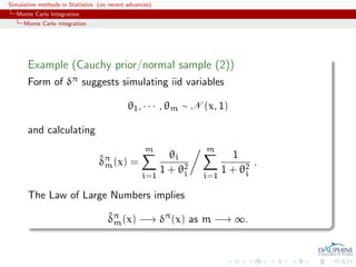
- 45. Simulation methods in Statistics (on recent advances) Monte Carlo Integration Monte Carlo integration Example (Cauchy prior/normal sample (2)) Form of δπ suggests simulating iid variables θ1 , · · · , θm ∼ N (x, 1) and calculating m m ˆm θi 1 δπ (x) = . 1 + θ2 i 1 + θ2 i i=1 i=1 The Law of Large Numbers implies δπ (x) −→ δπ (x) as m −→ ∞. ˆm
- 46. Simulation methods in Statistics (on recent advances) Monte Carlo Integration Monte Carlo integration 10.6 10.4 10.2 10.0 9.8 9.6 0 200 400 600 800 1000 iterations Range of estimators δπ for 100 runs and x = 10 m
- 47. Simulation methods in Statistics (on recent advances) Monte Carlo Integration Importance Sampling Importance sampling Paradox Simulation from f (the true density) is not necessarily optimal
- 48. Simulation methods in Statistics (on recent advances) Monte Carlo Integration Importance Sampling Importance sampling Paradox Simulation from f (the true density) is not necessarily optimal Alternative to direct sampling from f is importance sampling, based on the alternative representation f(x) Ef [h(X)] = h(x) g(x) dx . X g(x) which allows us to use other distributions than f
- 49. Simulation methods in Statistics (on recent advances) Monte Carlo Integration Importance Sampling Importance sampling algorithm Evaluation of Ef [h(X)] = h(x) f(x) dx X by 1 Generate a sample X1 , . . . , Xn from a distribution g 2 Use the approximation m 1 f(Xj ) h(Xj ) m g(Xj ) j=1
- 50. Simulation methods in Statistics (on recent advances) Monte Carlo Integration Importance Sampling Implementation details ◦ Instrumental distribution g chosen from distributions easy to simulate ◦ The same sample (generated from g) can be used repeatedly, not only for different functions h, but also for different densities f ◦ Dependent proposals can be used, as seen later Pop’MC
- 51. Simulation methods in Statistics (on recent advances) Monte Carlo Integration Importance Sampling Finite vs. infinite variance Although g can be any density, some choices are better than others: ◦ Finite variance only when f(X) f2 (X) Ef h2 (X) = h2 (x) dx < ∞ . g(X) X g(X)
- 52. Simulation methods in Statistics (on recent advances) Monte Carlo Integration Importance Sampling Finite vs. infinite variance Although g can be any density, some choices are better than others: ◦ Finite variance only when f(X) f2 (X) Ef h2 (X) = h2 (x) dx < ∞ . g(X) X g(X) ◦ Instrumental distributions with tails lighter than those of f (that is, with sup f/g = ∞) not appropriate. ◦ If sup f/g = ∞, the weights f(xj )/g(xj ) vary widely, giving too much importance to a few values xj .
- 53. Simulation methods in Statistics (on recent advances) Monte Carlo Integration Importance Sampling Finite vs. infinite variance Although g can be any density, some choices are better than others: ◦ Finite variance only when f(X) f2 (X) Ef h2 (X) = h2 (x) dx < ∞ . g(X) X g(X) ◦ Instrumental distributions with tails lighter than those of f (that is, with sup f/g = ∞) not appropriate. ◦ If sup f/g = ∞, the weights f(xj )/g(xj ) vary widely, giving too much importance to a few values xj . ◦ If sup f/g = M < ∞, finite variance for L2 functions
- 54. Simulation methods in Statistics (on recent advances) Monte Carlo Integration Importance Sampling Selfnormalised importance sampling For ratio estimator n n δn h = ωi h(xi ) ωi i=1 i=1 with Xi ∼ g(y) and Wi such that E[Wi |Xi = x] = κf(x)/g(x)
- 55. Simulation methods in Statistics (on recent advances) Monte Carlo Integration Importance Sampling Selfnormalised variance then 1 var(δn ) ≈ h var(Sn ) − 2Eπ [h] cov(Sn , Sn ) + Eπ [h]2 var(Sn ) . h h 1 1 n2 κ2 for n n Sn = h Wi h(Xi ) , Sn = 1 Wi i=1 i=1 Rough approximation 1 varδn ≈ h varπ (h(X)) {1 + varg (W)} n
- 56. Simulation methods in Statistics (on recent advances) Monte Carlo Integration Bayesian importance sampling Bayes factor approximation When approximating the Bayes factor f0 (x|θ0 )π0 (θ0 )dθ0 Θ0 B01 = f1 (x|θ1 )π1 (θ1 )dθ1 Θ1 use of importance functions 0 and 1 and n0 n−1 0 i i i=1 f0 (x|θ0 )π0 (θ0 )/ i 0 (θ0 ) B01 = n1 n−1 1 i i i=1 f1 (x|θ1 )π1 (θ1 )/ i 1 (θ1 )
- 57. Simulation methods in Statistics (on recent advances) Monte Carlo Integration Bayesian importance sampling Diabetes in Pima Indian women Example (R benchmark) “A population of women who were at least 21 years old, of Pima Indian heritage and living near Phoenix (AZ), was tested for diabetes according to WHO criteria. The data were collected by the US National Institute of Diabetes and Digestive and Kidney Diseases.” 200 Pima Indian women with observed variables plasma glucose concentration in oral glucose tolerance test diastolic blood pressure diabetes pedigree function presence/absence of diabetes
- 58. Simulation methods in Statistics (on recent advances) Monte Carlo Integration Bayesian importance sampling Probit modelling on Pima Indian women Probability of diabetes function of above variables P(y = 1|x) = Φ(x1 β1 + x2 β2 + x3 β3 ) ,
- 59. Simulation methods in Statistics (on recent advances) Monte Carlo Integration Bayesian importance sampling Probit modelling on Pima Indian women Probability of diabetes function of above variables P(y = 1|x) = Φ(x1 β1 + x2 β2 + x3 β3 ) , Test of H0 : β3 = 0 for 200 observations of Pima.tr based on a g-prior modelling: β ∼ N3 (0, n XT X)−1
- 60. Simulation methods in Statistics (on recent advances) Monte Carlo Integration Bayesian importance sampling Importance sampling for the Pima Indian dataset Use of the importance function inspired from the MLE estimate distribution β ∼ N(β, Σ) ˆ ˆ
- 61. Simulation methods in Statistics (on recent advances) Monte Carlo Integration Bayesian importance sampling Importance sampling for the Pima Indian dataset Use of the importance function inspired from the MLE estimate distribution β ∼ N(β, Σ) ˆ ˆ R Importance sampling code model1=summary(glm(y~-1+X1,family=binomial(link="probit"))) is1=rmvnorm(Niter,mean=model1$coeff[,1],sigma=2*model1$cov.unscaled) is2=rmvnorm(Niter,mean=model2$coeff[,1],sigma=2*model2$cov.unscaled) bfis=mean(exp(probitlpost(is1,y,X1)-dmvlnorm(is1,mean=model1$coeff[,1], sigma=2*model1$cov.unscaled))) / mean(exp(probitlpost(is2,y,X2)- dmvlnorm(is2,mean=model2$coeff[,1],sigma=2*model2$cov.unscaled)))
- 62. Simulation methods in Statistics (on recent advances) Monte Carlo Integration Bayesian importance sampling Diabetes in Pima Indian women Comparison of the variation of the Bayes factor approximations based on 100 replicas for 20, 000 simulations from the prior and the above MLE importance sampler 5 4 3 2 Basic Monte Carlo Importance sampling
- 63. Simulation methods in Statistics (on recent advances) Monte Carlo Integration Bayesian importance sampling Bridge sampling Special case: If π1 (θ1 |x) ∝ π1 (θ1 |x) ˜ π2 (θ2 |x) ∝ π2 (θ2 |x) ˜ live on the same space (Θ1 = Θ2 ), then n 1 π1 (θi |x) ˜ B12 ≈ θi ∼ π2 (θ|x) n π2 (θi |x) ˜ i=1 [Gelman & Meng, 1998; Chen, Shao & Ibrahim, 2000]
- 64. Simulation methods in Statistics (on recent advances) Monte Carlo Integration Bayesian importance sampling (Further) bridge sampling General identity: ˜ π2 (θ|x)α(θ)π1 (θ|x)dθ B12 = ∀ α(·) ˜ π1 (θ|x)α(θ)π2 (θ|x)dθ n1 1 π2 (θ1i |x)α(θ1i ) ˜ n1 ≈ i=1 n2 θji ∼ πj (θ|x) 1 π1 (θ2i |x)α(θ2i ) ˜ n2 i=1
- 65. Simulation methods in Statistics (on recent advances) Monte Carlo Integration Bayesian importance sampling Optimal bridge sampling The optimal choice of auxiliary function is n1 + n2 α = n1 π1 (θ|x) + n2 π2 (θ|x) leading to n1 1 π2 (θ1i |x) ˜ n1 n1 π1 (θ1i |x) + n2 π2 (θ1i |x) i=1 B12 ≈ n2 1 π1 (θ2i |x) ˜ n2 n1 π1 (θ2i |x) + n2 π2 (θ2i |x) i=1
- 66. Simulation methods in Statistics (on recent advances) Monte Carlo Integration Bayesian importance sampling Illustration for the Pima Indian dataset Use of the MLE induced conditional of β3 given (β1 , β2 ) as a pseudo-posterior and mixture of both MLE approximations on β3 in bridge sampling estimate
- 67. Simulation methods in Statistics (on recent advances) Monte Carlo Integration Bayesian importance sampling Illustration for the Pima Indian dataset Use of the MLE induced conditional of β3 given (β1 , β2 ) as a pseudo-posterior and mixture of both MLE approximations on β3 in bridge sampling estimate R bridge sampling code cova=model2$cov.unscaled expecta=model2$coeff[,1] covw=cova[3,3]-t(cova[1:2,3])%*%ginv(cova[1:2,1:2])%*%cova[1:2,3] probit1=hmprobit(Niter,y,X1) probit2=hmprobit(Niter,y,X2) pseudo=rnorm(Niter,meanw(probit1),sqrt(covw)) probit1p=cbind(probit1,pseudo) bfbs=mean(exp(probitlpost(probit2[,1:2],y,X1)+dnorm(probit2[,3],meanw(probit2[,1:2]), sqrt(covw),log=T))/ (dmvnorm(probit2,expecta,cova)+dnorm(probit2[,3],expecta[3], cova[3,3])))/ mean(exp(probitlpost(probit1p,y,X2))/(dmvnorm(probit1p,expecta,cova)+ dnorm(pseudo,expecta[3],cova[3,3])))
- 68. Simulation methods in Statistics (on recent advances) Monte Carlo Integration Bayesian importance sampling Diabetes in Pima Indian women (cont’d) Comparison of the variation of the Bayes factor approximations based on 100 × 20, 000 simulations from the prior (MC), the above bridge sampler and the above importance sampler
- 69. Simulation methods in Statistics (on recent advances) Monte Carlo Integration Bayesian importance sampling The original harmonic mean estimator When θki ∼ πk (θ|x), T 1 1 T L(θkt |x) t=1 is an unbiased estimator of 1/mk (x) [Newton & Raftery, 1994]
- 70. Simulation methods in Statistics (on recent advances) Monte Carlo Integration Bayesian importance sampling The original harmonic mean estimator When θki ∼ πk (θ|x), T 1 1 T L(θkt |x) t=1 is an unbiased estimator of 1/mk (x) [Newton & Raftery, 1994] Highly dangerous: Most often leads to an infinite variance!!!
- 71. Simulation methods in Statistics (on recent advances) Monte Carlo Integration Bayesian importance sampling “The Worst Monte Carlo Method Ever” “The good news is that the Law of Large Numbers guarantees that this estimator is consistent ie, it will very likely be very close to the correct answer if you use a sufficiently large number of points from the posterior distribution.
- 72. Simulation methods in Statistics (on recent advances) Monte Carlo Integration Bayesian importance sampling “The Worst Monte Carlo Method Ever” “The good news is that the Law of Large Numbers guarantees that this estimator is consistent ie, it will very likely be very close to the correct answer if you use a sufficiently large number of points from the posterior distribution. The bad news is that the number of points required for this estimator to get close to the right answer will often be greater than the number of atoms in the observable universe. The even worse news is that it’s easy for people to not realize this, and to na¨ıvely accept estimates that are nowhere close to the correct value of the marginal likelihood.” [Radford Neal’s blog, Aug. 23, 2008]
- 73. Simulation methods in Statistics (on recent advances) Monte Carlo Integration Bayesian importance sampling Approximating Zk from a posterior sample Use of the [harmonic mean] identity ϕ(θk ) ϕ(θk ) πk (θk )Lk (θk ) 1 Eπk x = dθk = πk (θk )Lk (θk ) πk (θk )Lk (θk ) Zk Zk no matter what the proposal ϕ(·) is. [Gelfand & Dey, 1994; Bartolucci et al., 2006]
- 74. Simulation methods in Statistics (on recent advances) Monte Carlo Integration Bayesian importance sampling Approximating Zk from a posterior sample Use of the [harmonic mean] identity ϕ(θk ) ϕ(θk ) πk (θk )Lk (θk ) 1 Eπk x = dθk = πk (θk )Lk (θk ) πk (θk )Lk (θk ) Zk Zk no matter what the proposal ϕ(·) is. [Gelfand & Dey, 1994; Bartolucci et al., 2006] Direct exploitation of the MCMC output
- 75. Simulation methods in Statistics (on recent advances) Monte Carlo Integration Bayesian importance sampling Comparison with regular importance sampling Harmonic mean: Constraint opposed to usual importance sampling constraints: ϕ(θ) must have lighter (rather than fatter) tails than πk (θk )Lk (θk ) for the approximation T (t) 1 ϕ(θk ) Z1k = 1 (t) (t) T πk (θk )Lk (θk ) t=1 to enjoy finite variance
- 76. Simulation methods in Statistics (on recent advances) Monte Carlo Integration Bayesian importance sampling Comparison with regular importance sampling (cont’d) Compare Z1k with a standard importance sampling approximation T (t) (t) 1 πk (θk )Lk (θk ) Z2k = (t) T ϕ(θk ) t=1 (t) where the θk ’s are generated from the density ϕ(·) (with fatter tails like t’s)
- 77. Simulation methods in Statistics (on recent advances) Monte Carlo Integration Bayesian importance sampling HPD indicator as ϕ Use the convex hull of MCMC simulations corresponding to the 10% HPD region (easily derived!) and ϕ as indicator: 10 ϕ(θ) = Id(θ,θ(t) ) T t∈HPD
- 78. Simulation methods in Statistics (on recent advances) Monte Carlo Integration Bayesian importance sampling Diabetes in Pima Indian women (cont’d) Comparison of the variation of the Bayes factor approximations based on 100 replicas for 20, 000 simulations for a simulation from the above harmonic mean sampler and importance samplers 3.102 3.104 3.106 3.108 3.110 3.112 3.114 3.116 Harmonic mean Importance sampling
- 79. Simulation methods in Statistics (on recent advances) Monte Carlo Integration Bayesian importance sampling Chib’s representation Direct application of Bayes’ theorem: given x ∼ fk (x|θk ) and θk ∼ πk (θk ), fk (x|θk ) πk (θk ) mk (x) = πk (θk |x) [Bayes Theorem]
- 80. Simulation methods in Statistics (on recent advances) Monte Carlo Integration Bayesian importance sampling Chib’s representation Direct application of Bayes’ theorem: given x ∼ fk (x|θk ) and θk ∼ πk (θk ), fk (x|θk ) πk (θk ) mk (x) = πk (θk |x) [Bayes Theorem] Use of an approximation to the posterior fk (x|θ∗ ) πk (θ∗ ) k k mk (x) = . πk (θ∗ |x) ˆ k
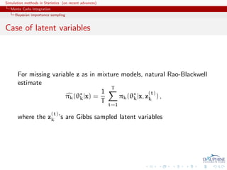
- 81. Simulation methods in Statistics (on recent advances) Monte Carlo Integration Bayesian importance sampling Case of latent variables For missing variable z as in mixture models, natural Rao-Blackwell estimate T ∗ 1 (t) πk (θk |x) = πk (θ∗ |x, zk ) , k T t=1 (t) where the zk ’s are Gibbs sampled latent variables
- 82. Simulation methods in Statistics (on recent advances) Monte Carlo Integration Bayesian importance sampling Case of the probit model For the completion by z, 1 ˆ π(θ|x) = π(θ|x, z(t) ) T t is a simple average of normal densities
- 83. Simulation methods in Statistics (on recent advances) Monte Carlo Integration Bayesian importance sampling Case of the probit model For the completion by z, 1 ˆ π(θ|x) = π(θ|x, z(t) ) T t is a simple average of normal densities R Bridge sampling code gibbs1=gibbsprobit(Niter,y,X1) gibbs2=gibbsprobit(Niter,y,X2) bfchi=mean(exp(dmvlnorm(t(t(gibbs2$mu)-model2$coeff[,1]),mean=rep(0,3), sigma=gibbs2$Sigma2)-probitlpost(model2$coeff[,1],y,X2)))/ mean(exp(dmvlnorm(t(t(gibbs1$mu)-model1$coeff[,1]),mean=rep(0,2), sigma=gibbs1$Sigma2)-probitlpost(model1$coeff[,1],y,X1)))
- 84. Simulation methods in Statistics (on recent advances) Monte Carlo Integration Bayesian importance sampling Diabetes in Pima Indian women (cont’d) Comparison of the variation of the Bayes factor approximations based on 100 replicas for 20, 000 simulations for a simulation from the above Chib’s and importance samplers
- 85. Simulation methods in Statistics (on recent advances) The Metropolis-Hastings Algorithm The Metropolis-Hastings Algorithm 1 Motivation and leading example 2 Monte Carlo Integration 3 The Metropolis-Hastings Algorithm Monte Carlo Methods based on Markov Chains The Metropolis–Hastings algorithm The random walk Metropolis-Hastings algorithm Adaptive MCMC 4 Approximate Bayesian computation
- 86. Simulation methods in Statistics (on recent advances) The Metropolis-Hastings Algorithm Monte Carlo Methods based on Markov Chains Running Monte Carlo via Markov Chains Epiphany! It is not necessary to use a sample from the distribution f to approximate the integral I= h(x)f(x)dx ,
- 87. Simulation methods in Statistics (on recent advances) The Metropolis-Hastings Algorithm Monte Carlo Methods based on Markov Chains Running Monte Carlo via Markov Chains Epiphany! It is not necessary to use a sample from the distribution f to approximate the integral I= h(x)f(x)dx , Principle: Obtain X1 , . . . , Xn ∼ f (approx) without directly simulating from f, using an ergodic Markov chain with stationary distribution f [Metropolis et al., 1953]
- 88. Simulation methods in Statistics (on recent advances) The Metropolis-Hastings Algorithm Monte Carlo Methods based on Markov Chains Running Monte Carlo via Markov Chains (2) Idea For an arbitrary starting value x(0) , an ergodic chain (X(t) ) is generated using a transition kernel with stationary distribution f
- 89. Simulation methods in Statistics (on recent advances) The Metropolis-Hastings Algorithm Monte Carlo Methods based on Markov Chains Running Monte Carlo via Markov Chains (2) Idea For an arbitrary starting value x(0) , an ergodic chain (X(t) ) is generated using a transition kernel with stationary distribution f Insures the convergence in distribution of (X(t) ) to a random variable from f. For a “large enough” T0 , X(T0 ) can be considered as distributed from f Produce a dependent sample X(T0 ) , X(T0 +1) , . . ., which is generated from f, sufficient for most approximation purposes.
- 90. Simulation methods in Statistics (on recent advances) The Metropolis-Hastings Algorithm Monte Carlo Methods based on Markov Chains Running Monte Carlo via Markov Chains (2) Idea For an arbitrary starting value x(0) , an ergodic chain (X(t) ) is generated using a transition kernel with stationary distribution f Insures the convergence in distribution of (X(t) ) to a random variable from f. For a “large enough” T0 , X(T0 ) can be considered as distributed from f Produce a dependent sample X(T0 ) , X(T0 +1) , . . ., which is generated from f, sufficient for most approximation purposes. Problem: How can one build a Markov chain with a given stationary distribution?
- 91. Simulation methods in Statistics (on recent advances) The Metropolis-Hastings Algorithm The Metropolis–Hastings algorithm The Metropolis–Hastings algorithm Basics The algorithm uses the objective (target) density f and a conditional density q(y|x) called the instrumental (or proposal) distribution
- 92. Simulation methods in Statistics (on recent advances) The Metropolis-Hastings Algorithm The Metropolis–Hastings algorithm The MH algorithm Algorithm (Metropolis–Hastings) Given x(t) , 1. Generate Yt ∼ q(y|x(t) ). 2. Take Yt with prob. ρ(x(t) , Yt ), X(t+1) = x(t) with prob. 1 − ρ(x(t) , Yt ), where f(y) q(x|y) ρ(x, y) = min ,1 . f(x) q(y|x)
- 93. Simulation methods in Statistics (on recent advances) The Metropolis-Hastings Algorithm The Metropolis–Hastings algorithm Features Independent of normalizing constants for both f and q(·|x) (ie, those constants independent of x) Never move to values with f(y) = 0 The chain (x(t) )t may take the same value several times in a row, even though f is a density wrt Lebesgue measure The sequence (yt )t is usually not a Markov chain
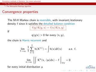
- 94. Simulation methods in Statistics (on recent advances) The Metropolis-Hastings Algorithm The Metropolis–Hastings algorithm Convergence properties The M-H Markov chain is reversible, with invariant/stationary density f since it satisfies the detailed balance condition f(y) K(y, x) = f(x) K(x, y)
- 95. Simulation methods in Statistics (on recent advances) The Metropolis-Hastings Algorithm The Metropolis–Hastings algorithm Convergence properties The M-H Markov chain is reversible, with invariant/stationary density f since it satisfies the detailed balance condition f(y) K(y, x) = f(x) K(x, y) If q(y|x) > 0 for every (x, y), the chain is Harris recurrent and T 1 lim h(X(t) ) = h(x)df(x) a.e. f. T →∞ T t=1 lim Kn (x, ·)µ(dx) − f =0 n→∞ TV for every initial distribution µ
- 96. Simulation methods in Statistics (on recent advances) The Metropolis-Hastings Algorithm The random walk Metropolis-Hastings algorithm Random walk Metropolis–Hastings Use of a local perturbation as proposal Yt = X(t) + εt , where εt ∼ g, independent of X(t) . The instrumental density is now of the form g(y − x) and the Markov chain is a random walk if we take g to be symmetric g(x) = g(−x)
- 97. Simulation methods in Statistics (on recent advances) The Metropolis-Hastings Algorithm The random walk Metropolis-Hastings algorithm Algorithm (Random walk Metropolis) Given x(t) 1 Generate Yt ∼ g(y − x(t) ) 2 Take Y f(Yt ) (t+1) t with prob. min 1, , X = f(x(t) ) x(t) otherwise.
- 98. Simulation methods in Statistics (on recent advances) The Metropolis-Hastings Algorithm The random walk Metropolis-Hastings algorithm RW-MH on mixture posterior distribution 3 2 µ2 1 0 X −1 −1 0 1 2 3 µ1 Random walk MCMC output for .7N(µ1 , 1) + .3N(µ2 , 1)
- 99. Simulation methods in Statistics (on recent advances) The Metropolis-Hastings Algorithm The random walk Metropolis-Hastings algorithm Acceptance rate A high acceptance rate is not indication of efficiency since the random walk may be moving “too slowly” on the target surface
- 100. Simulation methods in Statistics (on recent advances) The Metropolis-Hastings Algorithm The random walk Metropolis-Hastings algorithm Acceptance rate A high acceptance rate is not indication of efficiency since the random walk may be moving “too slowly” on the target surface If x(t) and yt are “too close”, i.e. f(x(t) ) f(yt ), yt is accepted with probability f(yt ) min ,1 1. f(x(t) ) and acceptance rate high
- 101. Simulation methods in Statistics (on recent advances) The Metropolis-Hastings Algorithm The random walk Metropolis-Hastings algorithm Acceptance rate A high acceptance rate is not indication of efficiency since the random walk may be moving “too slowly” on the target surface If average acceptance rate low, the proposed values f(yt ) tend to be small wrt f(x(t) ), i.e. the random walk [not the algorithm!] moves quickly on the target surface often reaching its boundaries
- 102. Simulation methods in Statistics (on recent advances) The Metropolis-Hastings Algorithm The random walk Metropolis-Hastings algorithm Rule of thumb In small dimensions, aim at an average acceptance rate of 50%. In large dimensions, at an average acceptance rate of 25%. [Gelman,Gilks and Roberts, 1995]
- 103. Simulation methods in Statistics (on recent advances) The Metropolis-Hastings Algorithm The random walk Metropolis-Hastings algorithm Noisy AR(1) Target distribution of x given x1 , x2 and y is −1 τ2 exp (x − ϕx1 )2 + (x2 − ϕx)2 + (y − x2 )2 . 2τ2 σ2 For a Gaussian random walk with scale ω small enough, the random walk never jumps to the other mode. But if the scale ω is sufficiently large, the Markov chain explores both modes and give a satisfactory approximation of the target distribution.
- 104. Simulation methods in Statistics (on recent advances) The Metropolis-Hastings Algorithm The random walk Metropolis-Hastings algorithm Noisy AR(2) Markov chain based on a random walk with scale ω = .1.
- 105. Simulation methods in Statistics (on recent advances) The Metropolis-Hastings Algorithm The random walk Metropolis-Hastings algorithm Noisy AR(3) Markov chain based on a random walk with scale ω = .5.
- 106. Simulation methods in Statistics (on recent advances) The Metropolis-Hastings Algorithm Adaptive MCMC No free lunch!! MCMC algorithm trained on-line usually invalid:
- 107. Simulation methods in Statistics (on recent advances) The Metropolis-Hastings Algorithm Adaptive MCMC No free lunch!! MCMC algorithm trained on-line usually invalid: using the whole past of the “chain” implies that this is not a Markov chain any longer!
- 108. Simulation methods in Statistics (on recent advances) The Metropolis-Hastings Algorithm Adaptive MCMC No free lunch!! MCMC algorithm trained on-line usually invalid: using the whole past of the “chain” implies that this is not a Markov chain any longer! This means standard Markov chain (ergodic) theory does not apply [Meyn & Tweedie, 1994]
- 109. Simulation methods in Statistics (on recent advances) The Metropolis-Hastings Algorithm Adaptive MCMC Example (Poly t distribution) t T(3, θ, 1) sample (x1 , . . . , xn ) with flat prior π(θ) = 1 Fit a normal proposal from empirical mean and empirical variance of the chain so far, t t 1 1 µt = θ(i) and σ2 t = (θ(i) − µt )2 , t t i=1 i=1
- 110. Simulation methods in Statistics (on recent advances) The Metropolis-Hastings Algorithm Adaptive MCMC Example (Poly t distribution) t T(3, θ, 1) sample (x1 , . . . , xn ) with flat prior π(θ) = 1 Fit a normal proposal from empirical mean and empirical variance of the chain so far, t t 1 1 µt = θ(i) and σ2 t = (θ(i) − µt )2 , t t i=1 i=1 Metropolis–Hastings algorithm with acceptance probability n −(ν+1)/2 ν + (xj − θ(t) )2 exp −(µt − θ(t) )2 /2σ2t , ν + (xj − ξ)2 exp −(µt − ξ)2 /2σ2 t j=2 where ξ ∼ N(µt , σ2 ). t
- 111. Simulation methods in Statistics (on recent advances) The Metropolis-Hastings Algorithm Adaptive MCMC Invalid scheme invariant distribution not invariant any longer when range of initial values too small, the θ(i) ’s cannot converge to the target distribution and concentrates on too small a support. long-range dependence on past values modifies the distribution of the sequence. using past simulations to create a non-parametric approximation to the target distribution does not work either
- 112. Simulation methods in Statistics (on recent advances) The Metropolis-Hastings Algorithm Adaptive MCMC 0.2 3 0.0 2 −0.2 x 1 −0.4 0 0 1000 2000 3000 4000 5000 −1.5 −1.0 −0.5 0.0 0.5 Iterations θ −1.5 −1.0 −0.5 0.0 0.5 1.0 1.5 0.6 0.4 x 0.2 0.0 0 1000 2000 3000 4000 5000 −2 −1 0 1 2 Iterations θ 0.0 0.1 0.2 0.3 0.4 0.5 0.6 0.7 2 1 0 x −1 −2 0 1000 2000 3000 4000 5000 −2 −1 0 1 2 3 Iterations θ Adaptive scheme for a sample of 10 xj ∼ T3 and initial variances of (top) 0.1, (middle) 0.5, and (bottom) 2.5.
- 113. Simulation methods in Statistics (on recent advances) The Metropolis-Hastings Algorithm Adaptive MCMC 1.0 1.5 0.8 1.0 0.6 0.5 x 0.4 0.0 0.2 −0.5 0.0 −1.0 0 10000 30000 50000 −1.5 −0.5 0.5 1.0 1.5 Iterations θ Sample produced by 50, 000 iterations of a nonparametric adaptive MCMC scheme and comparison of its distribution with the target distribution.
- 114. Simulation methods in Statistics (on recent advances) The Metropolis-Hastings Algorithm Adaptive MCMC Simply forget about it! Warning: One should not constantly adapt the proposal on past performances Either adaptation ceases after a period of burnin... or the adaptive scheme must be theoretically assessed on its own right. [Haario & Saaksman, 1999;Andrieu & Robert, 2001]
- 115. Simulation methods in Statistics (on recent advances) The Metropolis-Hastings Algorithm Adaptive MCMC Diminishing adaptation Adaptivity of cyberparameter γt has to be gradually tuned down to recover ergodicity [Roberts & Rosenthal, 2007]
- 116. Simulation methods in Statistics (on recent advances) The Metropolis-Hastings Algorithm Adaptive MCMC Diminishing adaptation Adaptivity of cyberparameter γt has to be gradually tuned down to recover ergodicity [Roberts & Rosenthal, 2007] Sufficient conditions: 1 total variation distance between two consecutive kernels must uniformly decrease to zero [diminishing adaptation] lim sup Kγt (x, ·) − Kγt+1 (x, ·) TV =0 t→∞ x 2 times to stationary remains bounded for any fixed γt [containment]
- 117. Simulation methods in Statistics (on recent advances) The Metropolis-Hastings Algorithm Adaptive MCMC Diminishing adaptation Adaptivity of cyberparameter γt has to be gradually tuned down to recover ergodicity [Roberts & Rosenthal, 2007] Sufficient conditions: 1 total variation distance between two consecutive kernels must uniformly decrease to zero [diminishing adaptation] lim sup Kγt (x, ·) − Kγt+1 (x, ·) TV =0 t→∞ x 2 times to stationary remains bounded for any fixed γt [containment] Works for random walk proposal that relies on the empirical variance of the sample modulo a ridge-like stabilizing factor [Haario, Sacksman & Tamminen, 1999]
- 118. Simulation methods in Statistics (on recent advances) The Metropolis-Hastings Algorithm Adaptive MCMC Diminishing adaptation Adaptivity of cyberparameter γt has to be gradually tuned down to recover ergodicity [Roberts & Rosenthal, 2007] Sufficient conditions: 1 total variation distance between two consecutive kernels must uniformly decrease to zero [diminishing adaptation] lim sup Kγt (x, ·) − Kγt+1 (x, ·) TV =0 t→∞ x 2 times to stationary remains bounded for any fixed γt [containment] Tune the scale in each direction toward an optimal acceptance rate of 0.44. [Roberts & Rosenthal,2006]
- 119. Simulation methods in Statistics (on recent advances) The Metropolis-Hastings Algorithm Adaptive MCMC Diminishing adaptation Adaptivity of cyberparameter γt has to be gradually tuned down to recover ergodicity [Roberts & Rosenthal, 2007] Sufficient conditions: 1 total variation distance between two consecutive kernels must uniformly decrease to zero [diminishing adaptation] lim sup Kγt (x, ·) − Kγt+1 (x, ·) TV =0 t→∞ x 2 times to stationary remains bounded for any fixed γt [containment] Packages amcmc and grapham
- 120. Simulation methods in Statistics (on recent advances) Approximate Bayesian computation Approximate Bayesian computation 1 Motivation and leading example 2 Monte Carlo Integration 3 The Metropolis-Hastings Algorithm 4 Approximate Bayesian computation ABC basics Alphabet soup Calibration of ABC
- 121. Simulation methods in Statistics (on recent advances) Approximate Bayesian computation ABC basics Untractable likelihoods There are cases when the likelihood function f(y|θ) is unavailable and when the completion step f(y|θ) = f(y, z|θ) dz Z is impossible or too costly because of the dimension of z c MCMC cannot be implemented! [Robert & Casella, 2004]
- 122. Simulation methods in Statistics (on recent advances) Approximate Bayesian computation ABC basics Illustrations Example Stochastic volatility model: for Highest weight trajectories t = 1, . . . , T , 0.4 0.2 yt = exp(zt ) t, zt = a+bzt−1 +σηt , 0.0 −0.2 T very large makes it difficult to −0.4 include z within the simulated 0 200 400 t 600 800 1000 parameters
- 123. Simulation methods in Statistics (on recent advances) Approximate Bayesian computation ABC basics Illustrations Example Potts model: if y takes values on a grid Y of size kn and f(y|θ) ∝ exp θ Iyl =yi l∼i where l∼i denotes a neighbourhood relation, n moderately large prohibits the computation of the normalising constant
- 124. Simulation methods in Statistics (on recent advances) Approximate Bayesian computation ABC basics Illustrations Example Inference on CMB: in cosmology, study of the Cosmic Microwave Background via likelihoods immensely slow to computate (e.g WMAP, Plank), because of numerically costly spectral transforms [Data is a Fortran program] [Kilbinger et al., 2010, MNRAS]
- 125. Simulation methods in Statistics (on recent advances) Approximate Bayesian computation ABC basics Illustrations Example Coalescence tree: in population genetics, reconstitution of a common ancestor from a sample of genes via a phylogenetic tree that is close to impossible to integrate out [100 processor days with 4 parameters] [Cornuet et al., 2009, Bioinformatics]
- 126. Simulation methods in Statistics (on recent advances) Approximate Bayesian computation ABC basics The ABC method Bayesian setting: target is π(θ)f(x|θ)
- 127. Simulation methods in Statistics (on recent advances) Approximate Bayesian computation ABC basics The ABC method Bayesian setting: target is π(θ)f(x|θ) When likelihood f(x|θ) not in closed form, likelihood-free rejection technique:
- 128. Simulation methods in Statistics (on recent advances) Approximate Bayesian computation ABC basics The ABC method Bayesian setting: target is π(θ)f(x|θ) When likelihood f(x|θ) not in closed form, likelihood-free rejection technique: ABC algorithm For an observation y ∼ f(y|θ), under the prior π(θ), keep jointly simulating θ ∼ π(θ) , z ∼ f(z|θ ) , until the auxiliary variable z is equal to the observed value, z = y. [Tavar´ et al., 1997] e
- 129. Simulation methods in Statistics (on recent advances) Approximate Bayesian computation ABC basics Why does it work?! The proof is trivial: f(θi ) ∝ π(θi )f(z|θi )Iy (z) z∈D ∝ π(θi )f(y|θi ) = π(θi |y) . [Accept–Reject 101]
- 130. Simulation methods in Statistics (on recent advances) Approximate Bayesian computation ABC basics Earlier occurrence ‘Bayesian statistics and Monte Carlo methods are ideally suited to the task of passing many models over one dataset’ [Don Rubin, Annals of Statistics, 1984] Note Rubin (1984) does not promote this algorithm for likelihood-free simulation but frequentist intuition on posterior distributions: parameters from posteriors are more likely to be those that could have generated the data.
- 131. Simulation methods in Statistics (on recent advances) Approximate Bayesian computation ABC basics A as approximative When y is a continuous random variable, equality z = y is replaced with a tolerance condition, ρ(y, z) where ρ is a distance
- 132. Simulation methods in Statistics (on recent advances) Approximate Bayesian computation ABC basics A as approximative When y is a continuous random variable, equality z = y is replaced with a tolerance condition, ρ(y, z) where ρ is a distance Output distributed from π(θ) Pθ {ρ(y, z) < } ∝ π(θ|ρ(y, z) < )
- 133. Simulation methods in Statistics (on recent advances) Approximate Bayesian computation ABC basics ABC algorithm Algorithm 1 Likelihood-free rejection sampler for i = 1 to N do repeat generate θ from the prior distribution π(·) generate z from the likelihood f(·|θ ) until ρ{η(z), η(y)} set θi = θ end for where η(y) defines a (maybe in-sufficient) statistic
- 134. Simulation methods in Statistics (on recent advances) Approximate Bayesian computation ABC basics Output The likelihood-free algorithm samples from the marginal in z of: π(θ)f(z|θ)IA ,y (z) π (θ, z|y) = , A ,y ×Θ π(θ)f(z|θ)dzdθ where A ,y = {z ∈ D|ρ(η(z), η(y)) < }.
- 135. Simulation methods in Statistics (on recent advances) Approximate Bayesian computation ABC basics Output The likelihood-free algorithm samples from the marginal in z of: π(θ)f(z|θ)IA ,y (z) π (θ, z|y) = , A ,y ×Θ π(θ)f(z|θ)dzdθ where A ,y = {z ∈ D|ρ(η(z), η(y)) < }. The idea behind ABC is that the summary statistics coupled with a small tolerance should provide a good approximation of the posterior distribution: π (θ|y) = π (θ, z|y)dz ≈ π(θ|y) .
- 136. Simulation methods in Statistics (on recent advances) Approximate Bayesian computation ABC basics Pima Indian benchmark 80 100 1.0 80 60 0.8 60 0.6 Density Density Density 40 40 0.4 20 20 0.2 0.0 0 0 −0.005 0.010 0.020 0.030 −0.05 −0.03 −0.01 −1.0 0.0 1.0 2.0 Figure: Comparison between density estimates of the marginals on β1 (left), β2 (center) and β3 (right) from ABC rejection samples (red) and MCMC samples (black) .
- 137. Simulation methods in Statistics (on recent advances) Approximate Bayesian computation ABC basics MA example Consider the MA(q) model q xt = t+ ϑi t−i i=1 Simple prior: uniform prior over the identifiability zone, e.g. triangle for MA(2)
- 138. Simulation methods in Statistics (on recent advances) Approximate Bayesian computation ABC basics MA example (2) ABC algorithm thus made of 1 picking a new value (ϑ1 , ϑ2 ) in the triangle 2 generating an iid sequence ( t )−q<t T 3 producing a simulated series (xt )1 t T
- 139. Simulation methods in Statistics (on recent advances) Approximate Bayesian computation ABC basics MA example (2) ABC algorithm thus made of 1 picking a new value (ϑ1 , ϑ2 ) in the triangle 2 generating an iid sequence ( t )−q<t T 3 producing a simulated series (xt )1 t T Distance: basic distance between the series T ρ((xt )1 t T , (xt )1 t T) = (xt − xt )2 t=1 or between summary statistics like the first q autocorrelations T τj = xt xt−j t=j+1
- 140. Simulation methods in Statistics (on recent advances) Approximate Bayesian computation ABC basics Comparison of distance impact Evaluation of the tolerance on the ABC sample against both distances ( = 100%, 10%, 1%, 0.1%) for an MA(2) model
- 141. Simulation methods in Statistics (on recent advances) Approximate Bayesian computation ABC basics Comparison of distance impact 4 1.5 3 1.0 2 0.5 1 0.0 0 0.0 0.2 0.4 0.6 0.8 −2.0 −1.0 0.0 0.5 1.0 1.5 θ1 θ2 Evaluation of the tolerance on the ABC sample against both distances ( = 100%, 10%, 1%, 0.1%) for an MA(2) model
- 142. Simulation methods in Statistics (on recent advances) Approximate Bayesian computation ABC basics Comparison of distance impact 4 1.5 3 1.0 2 0.5 1 0.0 0 0.0 0.2 0.4 0.6 0.8 −2.0 −1.0 0.0 0.5 1.0 1.5 θ1 θ2 Evaluation of the tolerance on the ABC sample against both distances ( = 100%, 10%, 1%, 0.1%) for an MA(2) model
- 143. Simulation methods in Statistics (on recent advances) Approximate Bayesian computation ABC basics ABC advances Simulating from the prior is often poor in efficiency
- 144. Simulation methods in Statistics (on recent advances) Approximate Bayesian computation ABC basics ABC advances Simulating from the prior is often poor in efficiency Either modify the proposal distribution on θ to increase the density of x’s within the vicinity of y... [Marjoram et al, 2003; Bortot et al., 2007, Sisson et al., 2007]
- 145. Simulation methods in Statistics (on recent advances) Approximate Bayesian computation ABC basics ABC advances Simulating from the prior is often poor in efficiency Either modify the proposal distribution on θ to increase the density of x’s within the vicinity of y... [Marjoram et al, 2003; Bortot et al., 2007, Sisson et al., 2007] ...or by viewing the problem as a conditional density estimation and by developing techniques to allow for larger [Beaumont et al., 2002]
- 146. Simulation methods in Statistics (on recent advances) Approximate Bayesian computation ABC basics ABC advances Simulating from the prior is often poor in efficiency Either modify the proposal distribution on θ to increase the density of x’s within the vicinity of y... [Marjoram et al, 2003; Bortot et al., 2007, Sisson et al., 2007] ...or by viewing the problem as a conditional density estimation and by developing techniques to allow for larger [Beaumont et al., 2002] .....or even by including in the inferential framework [ABCµ ] [Ratmann et al., 2009]
- 147. Simulation methods in Statistics (on recent advances) Approximate Bayesian computation Alphabet soup ABC-NP Better usage of [prior] simulations by adjustement: instead of throwing away θ such that ρ(η(z), η(y)) > , replace θs with locally regressed θ∗ = θ − {η(z) − η(y)}T β ˆ [Csill´ry et al., TEE, 2010] e ˆ where β is obtained by [NP] weighted least square regression on (η(z) − η(y)) with weights Kδ {ρ(η(z), η(y))} [Beaumont et al., 2002, Genetics]
- 148. Simulation methods in Statistics (on recent advances) Approximate Bayesian computation Alphabet soup ABC-MCMC Markov chain (θ(t) ) created via the transition function θ ∼ Kω (θ |θ(t) ) if x ∼ f(x|θ ) is such that x = y π(θ )Kω (t) |θ ) θ(t+1) = and u ∼ U(0, 1) π(θ(t) )K (θ |θ(t) ) , (t) ω (θ θ otherwise,
- 149. Simulation methods in Statistics (on recent advances) Approximate Bayesian computation Alphabet soup ABC-MCMC Markov chain (θ(t) ) created via the transition function θ ∼ Kω (θ |θ(t) ) if x ∼ f(x|θ ) is such that x = y π(θ )Kω (t) |θ ) θ(t+1) = and u ∼ U(0, 1) π(θ(t) )K (θ |θ(t) ) , (t) ω (θ θ otherwise, has the posterior π(θ|y) as stationary distribution [Marjoram et al, 2003]
- 150. Simulation methods in Statistics (on recent advances) Approximate Bayesian computation Alphabet soup ABC-MCMC (2) Algorithm 2 Likelihood-free MCMC sampler Use Algorithm 1 to get (θ(0) , z(0) ) for t = 1 to N do Generate θ from Kω ·|θ(t−1) , Generate z from the likelihood f(·|θ ), Generate u from U[0,1] , π(θ )Kω (θ(t−1) |θ ) if u I π(θ(t−1) Kω (θ |θ(t−1) ) A ,y (z ) then set (θ(t) , z(t) ) = (θ , z ) else (θ(t) , z(t) )) = (θ(t−1) , z(t−1) ), end if end for
- 151. Simulation methods in Statistics (on recent advances) Approximate Bayesian computation Alphabet soup Why does it work? Acceptance probability that does not involve the calculation of the likelihood and π (θ , z |y) Kω (θ(t−1) |θ )f(z(t−1) |θ(t−1) ) × π (θ(t−1) , z(t−1) |y) Kω (θ |θ(t−1) )f(z |θ ) π(θ ) f(z |θ ) IA ,y (z ) = (t−1) ) f(z(t−1) |θ(t−1) )I (t−1) ) π(θ A ,y (z Kω (θ(t−1) |θ ) f(z(t−1) |θ(t−1) ) × Kω (θ |θ(t−1) ) f(z |θ ) π(θ )Kω (θ(t−1) |θ ) = IA ,y (z ) . π(θ(t−1) Kω (θ |θ(t−1) )
- 152. Simulation methods in Statistics (on recent advances) Approximate Bayesian computation Alphabet soup ABCµ [Ratmann et al., 2009] Use of a joint density f(θ, |y) ∝ ξ( |y, θ) × πθ (θ) × π ( ) where y is the data, and ξ( |y, θ) is the prior predictive density of ρ(η(z), η(y)) given θ and x when z ∼ f(z|θ)
- 153. Simulation methods in Statistics (on recent advances) Approximate Bayesian computation Alphabet soup ABCµ [Ratmann et al., 2009] Use of a joint density f(θ, |y) ∝ ξ( |y, θ) × πθ (θ) × π ( ) where y is the data, and ξ( |y, θ) is the prior predictive density of ρ(η(z), η(y)) given θ and x when z ∼ f(z|θ) Warning! Replacement of ξ( |y, θ) with a non-parametric kernel approximation.
- 154. Simulation methods in Statistics (on recent advances) Approximate Bayesian computation Alphabet soup A PMC version Use of the same kernel idea as ABC-PRC but with IS correction [Beaumont et al., 2009; Toni et al., 2009] Generate a sample at iteration t by N (t−1) (t−1) ˆ πt (θ (t) )∝ ωj Kt (θ(t) |θj ) j=1 modulo acceptance of the associated xt , and use an importance (t) weight associated with an accepted simulation θi (t) (t) (t) ωi ∝ π(θi ) πt (θi ) . ˆ c Still likelihood-free [Beaumont et al., 2009]
- 155. Simulation methods in Statistics (on recent advances) Approximate Bayesian computation Alphabet soup Sequential Monte Carlo SMC is a simulation technique to approximate a sequence of related probability distributions πn with π0 “easy” and πT target. Iterated IS as PMC: particles moved from time n to time n via kernel Kn and use of a sequence of extended targets πn˜ n ˜ πn (z0:n ) = πn (zn ) Lj (zj+1 , zj ) j=0 where the Lj ’s are backward Markov kernels [check that πn (zn ) is a marginal] [Del Moral, Doucet & Jasra, 2006]
- 156. Simulation methods in Statistics (on recent advances) Approximate Bayesian computation Alphabet soup ABC-SMC True derivation of an SMC-ABC algorithm Use of a kernel Kn associated with target π n and derivation of the backward kernel π n (z )Kn (z , z) Ln−1 (z, z ) = πn (z) Update of the weights M m=1 IA n (xm ) in win ∝ wi(n−1) M m=1 IA n−1 (xm i(n−1) ) when xm ∼ K(xi(n−1) , ·) in
- 157. Simulation methods in Statistics (on recent advances) Approximate Bayesian computation Alphabet soup Properties of ABC-SMC The ABC-SMC method properly uses a backward kernel L(z, z ) to simplify the importance weight and to remove the dependence on the unknown likelihood from this weight. Update of importance weights is reduced to the ratio of the proportions of surviving particles Major assumption: the forward kernel K is supposed to be invariant against the true target [tempered version of the true posterior]
- 158. Simulation methods in Statistics (on recent advances) Approximate Bayesian computation Alphabet soup Properties of ABC-SMC The ABC-SMC method properly uses a backward kernel L(z, z ) to simplify the importance weight and to remove the dependence on the unknown likelihood from this weight. Update of importance weights is reduced to the ratio of the proportions of surviving particles Major assumption: the forward kernel K is supposed to be invariant against the true target [tempered version of the true posterior] Adaptivity in ABC-SMC algorithm only found in on-line construction of the thresholds t , slowly enough to keep a large number of accepted transitions [Del Moral, Doucet & Jasra, 2009]
- 159. Simulation methods in Statistics (on recent advances) Approximate Bayesian computation Calibration of ABC Which summary statistics? Fundamental difficulty of the choice of the summary statistic when there is no non-trivial sufficient statistic [except when done by the experimenters in the field]
- 160. Simulation methods in Statistics (on recent advances) Approximate Bayesian computation Calibration of ABC Which summary statistics? Fundamental difficulty of the choice of the summary statistic when there is no non-trivial sufficient statistic [except when done by the experimenters in the field] Starting from a large collection of summary statistics is available, Joyce and Marjoram (2008) consider the sequential inclusion into the ABC target, with a stopping rule based on a likelihood ratio test.
- 161. Simulation methods in Statistics (on recent advances) Approximate Bayesian computation Calibration of ABC Which summary statistics? Fundamental difficulty of the choice of the summary statistic when there is no non-trivial sufficient statistic [except when done by the experimenters in the field] Starting from a large collection of summary statistics is available, Joyce and Marjoram (2008) consider the sequential inclusion into the ABC target, with a stopping rule based on a likelihood ratio test. Does not taking into account the sequential nature of the tests Depends on parameterisation Order of inclusion matters.
- 162. Simulation methods in Statistics (on recent advances) Approximate Bayesian computation Calibration of ABC Point estimation vs.... In the case of the computation of E[h(θ)|y], Fearnhead and Prangle [12/14/2011] demonstrate that the optimal summary statistic is η (y) = E[h(θ)|y]
- 163. Simulation methods in Statistics (on recent advances) Approximate Bayesian computation Calibration of ABC Point estimation vs.... In the case of the computation of E[h(θ)|y], Fearnhead and Prangle [12/14/2011] demonstrate that the optimal summary statistic is η (y) = E[h(θ)|y] Unavailable but approximated by a prior ABC run and ABC-NP corrections
- 164. Simulation methods in Statistics (on recent advances) Approximate Bayesian computation Calibration of ABC ...vs. model choice In the case of the computation of a Bayes factor B12 (y), ABC approximation T T Im(t) =1 Im(t) =2 t=1 t=1 may fail to converge [Robert et al., 2011]
- 165. Simulation methods in Statistics (on recent advances) Approximate Bayesian computation Calibration of ABC ...vs. model choice In the case of the computation of a Bayes factor B12 (y), ABC approximation T T Im(t) =1 Im(t) =2 t=1 t=1 may fail to converge [Robert et al., 2011] Separation conditions on the summary statistics for convergence to occur [Marin et al., 2011]