SlideShare a Scribd company logo
Page | 1
Data Structure
M.Sc. Computer Science
I Semester
Ms. Arati Singh
Department of Computer Science
Shri Shankaracharya Mahavidyalaya Junwani Bhilai
Page | 2
UNIT-I
DataStructures&Algorithms-Overview
Data Structure is a systematic way to organize data in order to use it efficiently. Following terms
are the foundation terms of a data structure.
• Interface − Each data structure has an interface. Interface represents the set of operations
that a data structure supports. An interface only provides the list of supported operations,
type of parameters they can accept and return type of these operations.
• Implementation − Implementation provides the internal representation of a data structure.
Implementation also provides the definition of the algorithms used in the operations of the
data structure.
CharacteristicsofaDataStructure
• Correctness − Data structure implementation should implement its interface correctly.
• Time Complexity − Running time or the execution time of operations of data structure
must be as small as possible.
• Space Complexity − Memory usage of a data structure operation should be as little as
possible.
NeedforDataStructure
As applications are getting complex and data rich, there are three common problems that
applications face now-a-days.
• Data Search − Consider an inventory of 1 million (106
) items of a store. If the application
is to search an item, it has to search an item in 1 million (106
) items every time slowing
down the search. As data grows, search will become slower.
• Processor speed − Processor speed although being very high, falls limited if the data grows
to billion records.
• Multiple requests − As thousands of users can search data simultaneously on a web server,
even the fast server fails while searching the data.
To solve the above-mentioned problems, data structures come to rescue. Data can be organized in
a data structure in such a way that all items may not be required to be searched, and the required
data can be searched almost instantly
ExecutionTimeCases
There are three cases which are usually used to compare various data structure's execution time
in a relative manner.
• Worst Case − This is the scenario where a particular data structure operation takes maximum
time it can take. If an operation's worst case time is ƒ(n) then this operation will not take more
than ƒ(n) time where ƒ(n) represents function of n.
• Average Case − This is the scenario depicting the average execution time of an operation of a
data structure. If an operation takes ƒ(n) time in execution, then m operations will take mƒ(n)
time.
• Best Case − This is the scenario depicting the least possible execution time of an operation of a
data structure. If an operation takes ƒ(n) time in execution, then the actual operation may take
time as the random number which would be maximum as ƒ(n).
BasicTerminology
• Data − Data are values or set of values.
• Data Item − Data item refers to single unit of values.
• Group Items − Data items that are divided into sub items are called as Group Items.
• Elementary Items − Data items that cannot be divided are called as Elementary Items.
• Attribute and Entity − An entity is that which contains certain attributes or properties, which
may be assigned values.
• Entity Set − Entities of similar attributes form an entity set.
• Field − Field is a single elementary unit of information representing an attribute of an entity.
• Record − Record is a collection of field values of a given entity.
• File − File is a collection of records of the entities in a given entity set.
Data structure operation
Algorithm is a step-by-step procedure, which defines a set of instructions to be executed in a
certain order to get the desired output. Algorithms are generally created independent of
underlying languages, i.e. an algorithm can be implemented in more than one programming
language.
From the data structure point of view, following are some important categories of algorithms −
• Search − Algorithm to search an item in a data structure.
• Sort − Algorithm to sort items in a certain order.
• Insert − Algorithm to insert item in a data structure.
• Update − Algorithm to update an existing item in a data structure.
• Delete − Algorithm to delete an existing item from a data structure.
CharacteristicsofanAlgorithm
Not all procedures can be called an algorithm. An algorithm should have the following
characteristics −
• Unambiguous − Algorithm should be clear and unambiguous. Each of its steps (or phases), and
their inputs/outputs should be clear and must lead to only one meaning.
• Input − An algorithm should have 0 or more well-defined inputs.
• Output − An algorithm should have 1 or more well-defined outputs, and should match the
desired output.
• Finiteness − Algorithms must terminate after a finite number of steps.
• Feasibility − Should be feasible with the available resources.
• Independent − An algorithm should have step-by-step directions, which should be independent
of any programming code.
Hence, many solution algorithms can be derived for a given problem. The next step is to analyze
those proposed solution algorithms and implement the best suitable solution.
AlgorithmAnalysis
Efficiency of an algorithm can be analyzed at two different stages, before implementation and
after implementation. They are the following −
• A Priori Analysis − This is a theoretical analysis of an algorithm. Efficiency of an algorithm is
measured by assuming that all other factors, for example, processor speed, are constant and
have no effect on the implementation.
• A Posterior Analysis − This is an empirical analysis of an algorithm. The selected algorithm is
implemented using programming language. This is then executed on target computer machine.
In this analysis, actual statistics like running time and space required, are collected.
We shall learn about a priori algorithm analysis. Algorithm analysis deals with the execution or
running time of various operations involved. The running time of an operation can be defined as
the number of computer instructions executed per operation.
AlgorithmComplexity
Suppose X is an algorithm and n is the size of input data, the time and space used by the algorithm
X are the two main factors, which decide the efficiency of X.
• Time Factor − Time is measured by counting the number of key operations such as comparisons
in the sorting algorithm.
• Space Factor − Space is measured by counting the maximum memory space required by the
algorithm.
The complexity of an algorithm f(n) gives the running time and/or the storage space required by
the algorithm in terms of n as the size of input data.
SpaceComplexity
Space complexity of an algorithm represents the amount of memory space required by the algorithm
in its life cycle. The space required by an algorithm is equal to the sum of the following two
components −
• A fixed part that is a space required to store certain data and variables, that are independent of
the size of the problem. For example, simple variables and constants used, program size, etc.
• A variable part is a space required by variables, whose size depends on the size of the problem.
For example, dynamic memory allocation, recursion stack space, etc.
Space complexity S(P) of any algorithm P is S(P) = C + SP(I), where C is the fixed part and S(I) is
the variable part of the algorithm, which depends on instance characteristic I. Following is a simple
example that tries to explain the concept –
Algorithm: SUM(A, B)
Step 1 - START
Step 2 - C ← A + B + 10
Step 3 - Stop
Here we have three variables A, B, and C and one constant. Hence S(P) = 1 + 3. Now, space depends
on data types of given variables and constant types and it will be multiplied accordingly.
TimeComplexity
Time complexity of an algorithm represents the amount of time required by the algorithm to run to
completion. Time requirements can be defined as a numerical function T(n), where T(n) can be
measured as the number of steps, provided each step consumes constant time.
For example, addition of two n-bit integers takes n steps. Consequently, the total computational time
is T(n) = c ∗ n, where c is the time taken for the addition of two bits. Here, we observe that T(n) grows
linearly as the input size increases.
Sub-algorithms
◼ A sub-algorithm is a block of instructions that is executed when it is called from some other
point of the algorithm.
◼ The top-down algorithm design needs
- to write the sub-algorithm definitions
- to write an algorithm that calls the sub-algorithms
(i.e. includes a CALL statement for each one)
◼ Sub-algorithms are of two type:
- Sub-algorithms that do not return a value
- Sub-algorithms that return a value
* The sub-algorithm is called function in C++.
The Sub-algorithm Definition
a) Definition of a sub-algorithm that does not return a value
1- Sub-algorithm without arguments:
SUBALGORITHM subalgorithm-name ( )
Statements
END subalgorithm-name
where, ( ) is the empty list.
2- Sub-algorithm with arguments:
SUBALGORITHM subalgorithm-name (parameter-list)
Statements
END subalgorithm-name
where, Parameter-list is a list that contains one or more parameters that are passed to the sub-
algorithm.
DataStructures-AsymptoticAnalysis
Asymptotic analysis of an algorithm refers to defining the mathematical boundation/framing of its run-
time performance. Using asymptotic analysis, we can very well conclude the best case, average case,
and worst case scenario of an algorithm.
Asymptotic analysis is input bound i.e., if there's no input to the algorithm, it is concluded to work in
a constant time. Other than the "input" all other factors are considered constant.
Asymptotic analysis refers to computing the running time of any operation in mathematical units of
computation. For example, the running time of one operation is computed as f(n) and may be for another
operation it is computed as g(n2
). This means the first operation running time will increase linearly with
the increase in n and the running time of the second operation will increase exponentially
when n increases. Similarly, the running time of both operations will be nearly the same if n is
significantly small.
Usually, the time required by an algorithm falls under three types −
• Best Case − Minimum time required for program execution.
• Average Case − Average time required for program execution.
• Worst Case − Maximum time required for program execution.
AsymptoticNotations
Following are the commonly used asymptotic notations to calculate the running time complexity of an
algorithm.
• Ο Notation
• Ω Notation
• θ Notation
Big Oh Notation, Ο
The notation Ο(n) is the formal way to express the upper bound of an algorithm's running time. It
measures the worst case time complexity or the longest amount of time an algorithm can possibly take
to complete.
For example, for a function f(n)
Ο(f(n)) = {g(n): there exists c > 0 and n0 such that f(n) ≤ c.g(n) for all n > n0.}
Omega Notation, Ω
The notation Ω(n) is the formal way to express the lower bound of an algorithm's running time. It
measures the best case time complexity or the best amount of time an algorithm can possibly take to
complete.
For example, for a function f(n)
Ω(f(n)) ≥ { g(n) : there exists c > 0 and n0 such that g(n) ≤ c.f(n) for all n > n0. }
Theta Notation, θ
The notation θ(n) is the formal way to express both the lower bound and the upper bound of an
algorithm's running time. It is represented as follows −
θ(f(n)) = { g(n) if and only if g(n) = Ο(f(n)) and g(n) = Ω(f(n)) for all n > n0. }
CommonAsymptoticNotations
Following is a list of some common asymptotic notations −
constant − Ο(1)
logarithmic − Ο(log n)
linear − Ο(n)
n log n − Ο(n log n)
quadratic − Ο(n2
)
cubic − Ο(n3
)
polynomial − nΟ(1)
exponential − 2Ο(n)
Mathematical Notation and function
1. Floor and Ceiling Functions:
If x is a real number, then it means that x lies between two integers which are called the floor and
ceiling of x. i.e.
|_x_| is called the floor of x. It is the greatest integer that is not greater than x.
| x | is called the ceiling of x. It is the smallest integer that is not less than x.
If x is itself an integer, then |_x_| = | x |, otherwise |_x_| + 1 = | x | E.g.
|_3.14_|=3,|_-8.5_|=-9,|_7_|=7
| 3.14 |= 4, | -8.5 | = -8, | 7 |= 7
2. Remainder Function (Modular Arithmetic):
If k is any integer and M is a positive integer, then:
k (mod M)
gives the integer remainder when k is divided by M.
E.g.
25(mod7)=4
25(mod 5) = 0
3. Integer and Absolute Value Functions:
If x is a real number, then integer function INT(x) will convert x into integer and the fractional part
is removed.
E.g.
INT(3.14)=3
INT (-8.5) = -8
The absolute function ABS(x) or | x | gives the absolute value of x i.e. it gives the positive value of
x even if x is negative.
E.g.
ABS(-15)=15orABS|-15|=15
ABS(7)=7orABS7|=7
ABS(-3.33) = 3.33 or ABS | -3.33 | = 3.33
4. Summation Symbol (Sums):
The symbol which is used to denote summation is a Greek letter Sigma ?.
Let a1, a2, a3, ….. , an be a sequence of numbers. Then the sum a1 + a2 + a3 + ….. + an will be
written as:
n
? aj
j=1
where j is called the dummy index or dummy variable.
E.g.
n
?j=1+2+3+…..+n
j=1
5. Factorial Function:
n! denotes the product of the positive integers from 1 to n. n! is read as ‘n factorial’, i.e.
n! = 1 * 2 * 3 * ….. * (n-2) * (n-1) * n
E.g.
4!=1*2*3*4=24
5! = 5 * 4! = 120
6. Permutations:
Let we have a set of n elements. A permutation of this set means the arrangement of the elements
of the set in some order.
E.g.
Suppose the set contains a, b and c. The various permutations of these elements can be: abc, acb,
bac, bca, cab, cba.
If there are n elements in the set then there will be n! permutations of those elements. It means
if the set has 3 elements then there will be 3! = 1 * 2 * 3 = 6 permutations of the elements.
7. Exponents and Logarithms:
Exponent means how many times a number is multiplied by itself. If m is a positive integer, then:
am=a*a*a*…..*a(m times)
and
a-m=1/am
E.g.
24=2*2*2*2=16
2-4 = 1 / 24 = 1 / 16
Control structures
A control structure is a block of programming that analyzes variables and chooses a direction in
which to go based on given parameters. The term flow control details the direction the program
takes (which way program control "flows"). Hence it is the basic decision-making process in
computing; flow control determines how a computer will respond when given certain conditions
and parameters.
Basic Terminologies
Those initial conditions and parameters are called preconditions. Preconditions are the state of
variables before entering a control structure. Based on those preconditions, the computer runs
an algorithm (the control structure) to determine what to do. The result is called a post
condition. Post conditions are the state of variables after the algorithm is run.
An Example
Let us analyze flow control by using traffic flow as a model. A vehicle is arriving at an intersection.
Thus, the precondition is the vehicle is in motion. Suppose the traffic light at the intersection is red.
The control structure must determine the proper course of action to assign to the vehicle.
Precondition: The vehicle is in motion.
Treatments of Information through Control Structures
Is the traffic light green? If so, then the vehicle may stay in motion.
Is the traffic light red? If so, then the vehicle must stop.
End of Treatment
Post condition: The vehicle comes to a stop.
Thus, upon exiting the control structure, the vehicle is stopped.
can also be form as a structure
IF-THEN Statement[edit]
The IF-THEN statement is a simple control that tests whether a condition is true or false. The
condition can include a variable, or be a variable. If the variable is an integer 2, it will be true,
because any number that is not zero will be true. If the condition is true, then an action occurs. If
the condition is false, nothing is done. To illustrate:
IF variable is true
THEN take this course of action.
If the variable indeed holds a value consistent with being true, then the course of action is taken. If
the variable is not true, then there is no course of action taken.
IF-THEN-ELSE Statement
IF-THEN statements test for only one action. With an IF-THEN-ELSE statement, the control can
"look both ways" so to speak, and take a secondary course of action. If the condition is true, then
an action occurs. If the condition is false, take an alternate action. To illustrate:
IF variable is true
THEN take this course of action
ELSE call another routine
In this case, if the variable is true, it takes a certain course of action and completely skips the ELSE
clause. If the variable is false, the control structure calls a routine and completely skips the THEN
clause.
Note that you can combine ELSE's with other IF's, allowing several tests to be made. In an IF-
THEN-ELSEIF-THEN-ELSEIF-THEN-ELSEIF-THEN structure, tests will stop as soon as a
condition is true. That's why you'd probably want to put the most "likely" test first, for efficiency
(Remembering that ELSE's are skipped if the first condition is true, meaning that the remaining
portions of the IF-THEN-ELSEIF... would not be processed).
eg:
In case your computer doesn't start
IF a floppy disk is in the drive
THEN remove it and restart
ELSE IF you don't have any OS installed
THEN install an OS
ELSE call the hotline
You can have as many ELSE IF's as you like.
WHILE and DO-WHILE Loops
A WHILE loop is a process in which a loop is initiated until a condition has been met. This structure
is useful when performing iterative instructions to satisfy a certain parameter. To illustrate:
Precondition: variable X is equal to 1
WHILE X is not equal to 9
Add 1 to X
This routine will add 1 to X until X is equal to 9, at which point the control structure will quit and
move on to the next instruction. Note that when the structure quits, it will not execute the Add
function: when X is equal to 9, it will skip over the clause that is attached to the WHILE. This
instruction is useful if a parameter needs to be tested repeatedly before acceptance.
DO-WHILE Loops
A DO-WHILE loop is nearly the exact opposite to a WHILE loop. A WHILE loop initially checks
to see if the parameters have been satisfied before executing an instruction. A DO-WHILE loop
executes the instruction before checking the parameters. To illustrate:
DO Add 1 to X
WHILE X is not equal 9
As you can see, the example differs from the first illustration, where the DO action is taken before
the WHILE. The WHILE is inclusive in the DO. As such, if the WHILE results in a false (X is
equal to 9), the control structure will break and will not perform another DO. Note that if X is equal
to or greater than 9 prior to entering the DO-WHILE loop, then the loop will never terminate.
FOR Loops
A FOR loop is an extension of a while loop. A for loop usually has three commands. The first is
used to set a starting point (like x = 0). The second is the end condition (same as in a while loop)
and is run every round. The third is also run every round and is usually used to modify a value used
in the condition block.
FOR X is 0. X is less than 10. add 1 to X.
This loop would be run 10 times (x being 0 to 9) so you won't have to think about the X variable in
the loop you can just put code there. Here is a while loop that does the same:
X is 0
WHILE X is less than 10
add 1 to X
Some programming languages also have a foreach loop which will be useful when working with
arrays (and collections). A foreach loop is an even more automated while loop that cycles through
array's and such. Example :
FOREACH student IN students
give a good mark to student
DataStructures&AlgorithmBasicConcepts
DataDefinition
Data Definition defines a particular data with the following characteristics.
• Atomic − Definition should define a single concept.
• Traceable − Definition should be able to be mapped to some data element.
• Accurate − Definition should be unambiguous.
• Clear and Concise − Definition should be understandable.
DataObject
Data Object represents an object having a data.
DataType
Data type is a way to classify various types of data such as integer, string, etc. which determines
the values that can be used with the corresponding type of data, the type of operations that can be
performed on the corresponding type of data. There are two data types −
• Built-in Data Type
• Derived Data Type
Built-in Data Type
Those data types for which a language has built-in support are known as Built-in Data types. For
example, most of the languages provide the following built-in data types.
• Integers
• Boolean (true, false)
• Floating (Decimal numbers)
• Character and Strings
Derived Data Type
Those data types which are implementation independent as they can be implemented in one or the
other way are known as derived data types. These data types are normally built by the combination
of primary or built-in data types and associated operations on them. For example −
• List
• Array
• Stack
• Queue
Reference
https://keithlyons.me/blog/2018/11/07/el30-graphing/
https://www.tutorialspoint.com/data_structures_algorithms/index.htm
https://www.geeksforgeeks.org/data-structures/
U nit   i data structure-converted

More Related Content

What's hot (20)

PPT
Data structure lecture 2
Kumar
 
PPTX
Data structures
Sneha Chopra
 
PPT
Introduction of data structure
eShikshak
 
PPTX
Searching Algorithms
Afaq Mansoor Khan
 
PPTX
Data structures and algorithms
Julie Iskander
 
PDF
BCA DATA STRUCTURES LINEAR ARRAYS MRS.SOWMYA JYOTHI
Sowmya Jyothi
 
PPT
Data Structure In C#
Shahzad
 
PPTX
Data Structure and Algorithms
Sumathi MathanMohan
 
PPT
Cis435 week04
ashish bansal
 
PPTX
Dynamic Memory & Linked Lists
Afaq Mansoor Khan
 
PPTX
Data structures in c#
SivaSankar Gorantla
 
PDF
DATA STRUCTURE AND ALGORITHM FULL NOTES
Aniruddha Paul
 
PDF
Introduction to Data Structure
Prof Ansari
 
PPT
Data Structures- Part1 overview and review
Abdullah Al-hazmy
 
PPTX
Introduction to data_structure
Ashim Lamichhane
 
PDF
BCA DATA STRUCTURES ALGORITHMS AND PRELIMINARIES MRS SOWMYA JYOTHI
Sowmya Jyothi
 
PDF
Algorithms Lecture 6: Searching Algorithms
Mohamed Loey
 
PDF
Data structure ppt
Prof. Dr. K. Adisesha
 
PDF
Data Structures (BE)
PRABHAHARAN429
 
PPT
Arrays Data Structure
student
 
Data structure lecture 2
Kumar
 
Data structures
Sneha Chopra
 
Introduction of data structure
eShikshak
 
Searching Algorithms
Afaq Mansoor Khan
 
Data structures and algorithms
Julie Iskander
 
BCA DATA STRUCTURES LINEAR ARRAYS MRS.SOWMYA JYOTHI
Sowmya Jyothi
 
Data Structure In C#
Shahzad
 
Data Structure and Algorithms
Sumathi MathanMohan
 
Cis435 week04
ashish bansal
 
Dynamic Memory & Linked Lists
Afaq Mansoor Khan
 
Data structures in c#
SivaSankar Gorantla
 
DATA STRUCTURE AND ALGORITHM FULL NOTES
Aniruddha Paul
 
Introduction to Data Structure
Prof Ansari
 
Data Structures- Part1 overview and review
Abdullah Al-hazmy
 
Introduction to data_structure
Ashim Lamichhane
 
BCA DATA STRUCTURES ALGORITHMS AND PRELIMINARIES MRS SOWMYA JYOTHI
Sowmya Jyothi
 
Algorithms Lecture 6: Searching Algorithms
Mohamed Loey
 
Data structure ppt
Prof. Dr. K. Adisesha
 
Data Structures (BE)
PRABHAHARAN429
 
Arrays Data Structure
student
 

Similar to U nit i data structure-converted (20)

PDF
Chapter 1 Introduction to Data Structures and Algorithms.pdf
Axmedcarb
 
PPTX
Chapter 1 Data structure _Algorithms.pptx
BifaHirpo1
 
PDF
Unit 1 OF DS FOR AI DS BTRCH OF DS FOR AI DS BTRCH .pdf
prathamsingh33
 
PPTX
FALLSEM2022-23_BCSE202L_TH_VL2022230103292_Reference_Material_I_25-07-2022_Fu...
AntareepMajumder
 
PDF
Data structures and algorithms Module-1.pdf
DukeCalvin
 
PPTX
Chapter 1 - Introduction to data structure.pptx
gadisaAdamu
 
DOCX
3rd-Sem_CSE_Data-Structures and Applications.docx
harshavardhan543715
 
PPTX
Unit I- Data structures Introduction, Evaluation of Algorithms, Arrays, Spars...
DrkhanchanaR
 
PPTX
Intro to Data Structure & Algorithms
Akhil Kaushik
 
PPTX
Data Structures - Lecture 1 - Unit 1.pptx
DanielNesaKumarC
 
DOCX
Data Structure Notes unit 1.docx
kp370932
 
PPT
assignment character education assignment
tsegayeblen57
 
PPT
Data Structure and Algorithm chapter two, This material is for Data Structure...
bekidea
 
PPTX
Introduction to Data Structure and algorithm.pptx
esuEthopi
 
PPTX
Basic of Data Structure - Data Structure - Notes
Omprakash Chauhan
 
PPTX
Data strucutre basic introduction
manirajan12
 
PPTX
data structure and algoriythm pres.pptxD
dubaay100
 
PDF
Data_structure using C-Adi.pdf
Prof. Dr. K. Adisesha
 
PPTX
MD AZAM CA-1-1.pptx
MyMovies15
 
Chapter 1 Introduction to Data Structures and Algorithms.pdf
Axmedcarb
 
Chapter 1 Data structure _Algorithms.pptx
BifaHirpo1
 
Unit 1 OF DS FOR AI DS BTRCH OF DS FOR AI DS BTRCH .pdf
prathamsingh33
 
FALLSEM2022-23_BCSE202L_TH_VL2022230103292_Reference_Material_I_25-07-2022_Fu...
AntareepMajumder
 
Data structures and algorithms Module-1.pdf
DukeCalvin
 
Chapter 1 - Introduction to data structure.pptx
gadisaAdamu
 
3rd-Sem_CSE_Data-Structures and Applications.docx
harshavardhan543715
 
Unit I- Data structures Introduction, Evaluation of Algorithms, Arrays, Spars...
DrkhanchanaR
 
Intro to Data Structure & Algorithms
Akhil Kaushik
 
Data Structures - Lecture 1 - Unit 1.pptx
DanielNesaKumarC
 
Data Structure Notes unit 1.docx
kp370932
 
assignment character education assignment
tsegayeblen57
 
Data Structure and Algorithm chapter two, This material is for Data Structure...
bekidea
 
Introduction to Data Structure and algorithm.pptx
esuEthopi
 
Basic of Data Structure - Data Structure - Notes
Omprakash Chauhan
 
Data strucutre basic introduction
manirajan12
 
data structure and algoriythm pres.pptxD
dubaay100
 
Data_structure using C-Adi.pdf
Prof. Dr. K. Adisesha
 
MD AZAM CA-1-1.pptx
MyMovies15
 
Ad

More from Shri Shankaracharya College, Bhilai,Junwani (20)

PPT
Environment Economics &Ethics invisible hand & Malthusian theory
Shri Shankaracharya College, Bhilai,Junwani
 
PPT
Azadi ka amrut mahotsav, Mahilayon ka yogdan swatantrata Sangram mein
Shri Shankaracharya College, Bhilai,Junwani
 
PDF
B.ed 1,scientific temper
Shri Shankaracharya College, Bhilai,Junwani
 
PDF
Aims and objectives of bio. sci. 14 9-20
Shri Shankaracharya College, Bhilai,Junwani
 
PPTX
Ict application in bio.sc.24 9
Shri Shankaracharya College, Bhilai,Junwani
 
PPTX
Isolation & preservation of culture of microorganism
Shri Shankaracharya College, Bhilai,Junwani
 
PPTX
Learners understanding,unit 1, 15-9-20
Shri Shankaracharya College, Bhilai,Junwani
 
PPTX
Basics concept of physical chemistry
Shri Shankaracharya College, Bhilai,Junwani
 
Ad

Recently uploaded (20)

PPTX
Systamatic Acquired Resistence (SAR).pptx
giriprasanthmuthuraj
 
PPTX
LESSON 2 PSYCHOSOCIAL DEVELOPMENT.pptx L
JeanCarolColico1
 
PDF
BlackBody Radiation experiment report.pdf
Ghadeer Shaabna
 
PDF
soil and environmental microbiology.pdf
Divyaprabha67
 
PDF
Service innovation with AI: Transformation of value proposition and market se...
Selcen Ozturkcan
 
PDF
Carbonate formation and fluctuating habitability on Mars
Sérgio Sacani
 
PDF
Adding Geochemistry To Understand Recharge Areas - Kinney County, Texas - Jim...
Texas Alliance of Groundwater Districts
 
PDF
Carbon-richDustInjectedintotheInterstellarMediumbyGalacticWCBinaries Survives...
Sérgio Sacani
 
PDF
Unit-5 ppt.pdf unit 5 organic chemistry 3
visionshukla007
 
PDF
Portable Hyperspectral Imaging (pHI) for the enhanced recording of archaeolog...
crabbn
 
PPTX
Basal_ganglia_Structure_Function_Importance
muralinath2
 
PDF
Global Congress on Forensic Science and Research
infoforensicscience2
 
PDF
Plant growth promoting bacterial non symbiotic
psuvethapalani
 
PDF
A Man of the Forest: The Contributions of Gifford Pinchot
RowanSales
 
PPTX
Ghent University Global Campus: Overview
Ghent University Global Campus
 
DOCX
Critical Book Review (CBR) - "Hate Speech: Linguistic Perspectives"
Sahmiral Amri Rajagukguk
 
PDF
The ALMA-CRISTAL survey: Gas, dust, and stars in star-forming galaxies when t...
Sérgio Sacani
 
PDF
Asthamudi lake and its fisheries&importance .pdf
J. Bovas Joel BFSc
 
PPTX
Phage Therapy and Bacteriophage Biology.pptx
Prachi Virat
 
PPTX
Diagnostic Features of Common Oral Ulcerative Lesions.pptx
Dr Palak borade
 
Systamatic Acquired Resistence (SAR).pptx
giriprasanthmuthuraj
 
LESSON 2 PSYCHOSOCIAL DEVELOPMENT.pptx L
JeanCarolColico1
 
BlackBody Radiation experiment report.pdf
Ghadeer Shaabna
 
soil and environmental microbiology.pdf
Divyaprabha67
 
Service innovation with AI: Transformation of value proposition and market se...
Selcen Ozturkcan
 
Carbonate formation and fluctuating habitability on Mars
Sérgio Sacani
 
Adding Geochemistry To Understand Recharge Areas - Kinney County, Texas - Jim...
Texas Alliance of Groundwater Districts
 
Carbon-richDustInjectedintotheInterstellarMediumbyGalacticWCBinaries Survives...
Sérgio Sacani
 
Unit-5 ppt.pdf unit 5 organic chemistry 3
visionshukla007
 
Portable Hyperspectral Imaging (pHI) for the enhanced recording of archaeolog...
crabbn
 
Basal_ganglia_Structure_Function_Importance
muralinath2
 
Global Congress on Forensic Science and Research
infoforensicscience2
 
Plant growth promoting bacterial non symbiotic
psuvethapalani
 
A Man of the Forest: The Contributions of Gifford Pinchot
RowanSales
 
Ghent University Global Campus: Overview
Ghent University Global Campus
 
Critical Book Review (CBR) - "Hate Speech: Linguistic Perspectives"
Sahmiral Amri Rajagukguk
 
The ALMA-CRISTAL survey: Gas, dust, and stars in star-forming galaxies when t...
Sérgio Sacani
 
Asthamudi lake and its fisheries&importance .pdf
J. Bovas Joel BFSc
 
Phage Therapy and Bacteriophage Biology.pptx
Prachi Virat
 
Diagnostic Features of Common Oral Ulcerative Lesions.pptx
Dr Palak borade
 

U nit i data structure-converted

  • 1. Page | 1 Data Structure M.Sc. Computer Science I Semester Ms. Arati Singh Department of Computer Science Shri Shankaracharya Mahavidyalaya Junwani Bhilai
  • 2. Page | 2 UNIT-I DataStructures&Algorithms-Overview Data Structure is a systematic way to organize data in order to use it efficiently. Following terms are the foundation terms of a data structure. • Interface − Each data structure has an interface. Interface represents the set of operations that a data structure supports. An interface only provides the list of supported operations, type of parameters they can accept and return type of these operations. • Implementation − Implementation provides the internal representation of a data structure. Implementation also provides the definition of the algorithms used in the operations of the data structure. CharacteristicsofaDataStructure • Correctness − Data structure implementation should implement its interface correctly. • Time Complexity − Running time or the execution time of operations of data structure must be as small as possible. • Space Complexity − Memory usage of a data structure operation should be as little as possible. NeedforDataStructure As applications are getting complex and data rich, there are three common problems that applications face now-a-days. • Data Search − Consider an inventory of 1 million (106 ) items of a store. If the application is to search an item, it has to search an item in 1 million (106 ) items every time slowing down the search. As data grows, search will become slower. • Processor speed − Processor speed although being very high, falls limited if the data grows to billion records. • Multiple requests − As thousands of users can search data simultaneously on a web server, even the fast server fails while searching the data. To solve the above-mentioned problems, data structures come to rescue. Data can be organized in a data structure in such a way that all items may not be required to be searched, and the required data can be searched almost instantly
  • 3. ExecutionTimeCases There are three cases which are usually used to compare various data structure's execution time in a relative manner. • Worst Case − This is the scenario where a particular data structure operation takes maximum time it can take. If an operation's worst case time is ƒ(n) then this operation will not take more than ƒ(n) time where ƒ(n) represents function of n. • Average Case − This is the scenario depicting the average execution time of an operation of a data structure. If an operation takes ƒ(n) time in execution, then m operations will take mƒ(n) time. • Best Case − This is the scenario depicting the least possible execution time of an operation of a data structure. If an operation takes ƒ(n) time in execution, then the actual operation may take time as the random number which would be maximum as ƒ(n). BasicTerminology • Data − Data are values or set of values. • Data Item − Data item refers to single unit of values. • Group Items − Data items that are divided into sub items are called as Group Items. • Elementary Items − Data items that cannot be divided are called as Elementary Items. • Attribute and Entity − An entity is that which contains certain attributes or properties, which may be assigned values. • Entity Set − Entities of similar attributes form an entity set. • Field − Field is a single elementary unit of information representing an attribute of an entity. • Record − Record is a collection of field values of a given entity. • File − File is a collection of records of the entities in a given entity set.
  • 4. Data structure operation Algorithm is a step-by-step procedure, which defines a set of instructions to be executed in a certain order to get the desired output. Algorithms are generally created independent of underlying languages, i.e. an algorithm can be implemented in more than one programming language. From the data structure point of view, following are some important categories of algorithms − • Search − Algorithm to search an item in a data structure. • Sort − Algorithm to sort items in a certain order. • Insert − Algorithm to insert item in a data structure. • Update − Algorithm to update an existing item in a data structure. • Delete − Algorithm to delete an existing item from a data structure. CharacteristicsofanAlgorithm Not all procedures can be called an algorithm. An algorithm should have the following characteristics − • Unambiguous − Algorithm should be clear and unambiguous. Each of its steps (or phases), and their inputs/outputs should be clear and must lead to only one meaning. • Input − An algorithm should have 0 or more well-defined inputs. • Output − An algorithm should have 1 or more well-defined outputs, and should match the desired output. • Finiteness − Algorithms must terminate after a finite number of steps. • Feasibility − Should be feasible with the available resources. • Independent − An algorithm should have step-by-step directions, which should be independent of any programming code. Hence, many solution algorithms can be derived for a given problem. The next step is to analyze those proposed solution algorithms and implement the best suitable solution.
  • 5. AlgorithmAnalysis Efficiency of an algorithm can be analyzed at two different stages, before implementation and after implementation. They are the following − • A Priori Analysis − This is a theoretical analysis of an algorithm. Efficiency of an algorithm is measured by assuming that all other factors, for example, processor speed, are constant and have no effect on the implementation. • A Posterior Analysis − This is an empirical analysis of an algorithm. The selected algorithm is implemented using programming language. This is then executed on target computer machine. In this analysis, actual statistics like running time and space required, are collected. We shall learn about a priori algorithm analysis. Algorithm analysis deals with the execution or running time of various operations involved. The running time of an operation can be defined as the number of computer instructions executed per operation. AlgorithmComplexity Suppose X is an algorithm and n is the size of input data, the time and space used by the algorithm X are the two main factors, which decide the efficiency of X. • Time Factor − Time is measured by counting the number of key operations such as comparisons in the sorting algorithm. • Space Factor − Space is measured by counting the maximum memory space required by the algorithm. The complexity of an algorithm f(n) gives the running time and/or the storage space required by the algorithm in terms of n as the size of input data. SpaceComplexity Space complexity of an algorithm represents the amount of memory space required by the algorithm in its life cycle. The space required by an algorithm is equal to the sum of the following two components − • A fixed part that is a space required to store certain data and variables, that are independent of the size of the problem. For example, simple variables and constants used, program size, etc. • A variable part is a space required by variables, whose size depends on the size of the problem. For example, dynamic memory allocation, recursion stack space, etc. Space complexity S(P) of any algorithm P is S(P) = C + SP(I), where C is the fixed part and S(I) is the variable part of the algorithm, which depends on instance characteristic I. Following is a simple example that tries to explain the concept –
  • 6. Algorithm: SUM(A, B) Step 1 - START Step 2 - C ← A + B + 10 Step 3 - Stop Here we have three variables A, B, and C and one constant. Hence S(P) = 1 + 3. Now, space depends on data types of given variables and constant types and it will be multiplied accordingly. TimeComplexity Time complexity of an algorithm represents the amount of time required by the algorithm to run to completion. Time requirements can be defined as a numerical function T(n), where T(n) can be measured as the number of steps, provided each step consumes constant time. For example, addition of two n-bit integers takes n steps. Consequently, the total computational time is T(n) = c ∗ n, where c is the time taken for the addition of two bits. Here, we observe that T(n) grows linearly as the input size increases. Sub-algorithms ◼ A sub-algorithm is a block of instructions that is executed when it is called from some other point of the algorithm. ◼ The top-down algorithm design needs - to write the sub-algorithm definitions - to write an algorithm that calls the sub-algorithms (i.e. includes a CALL statement for each one) ◼ Sub-algorithms are of two type: - Sub-algorithms that do not return a value - Sub-algorithms that return a value * The sub-algorithm is called function in C++.
  • 7. The Sub-algorithm Definition a) Definition of a sub-algorithm that does not return a value 1- Sub-algorithm without arguments: SUBALGORITHM subalgorithm-name ( ) Statements END subalgorithm-name where, ( ) is the empty list. 2- Sub-algorithm with arguments: SUBALGORITHM subalgorithm-name (parameter-list) Statements END subalgorithm-name where, Parameter-list is a list that contains one or more parameters that are passed to the sub- algorithm. DataStructures-AsymptoticAnalysis Asymptotic analysis of an algorithm refers to defining the mathematical boundation/framing of its run- time performance. Using asymptotic analysis, we can very well conclude the best case, average case, and worst case scenario of an algorithm. Asymptotic analysis is input bound i.e., if there's no input to the algorithm, it is concluded to work in a constant time. Other than the "input" all other factors are considered constant. Asymptotic analysis refers to computing the running time of any operation in mathematical units of computation. For example, the running time of one operation is computed as f(n) and may be for another operation it is computed as g(n2 ). This means the first operation running time will increase linearly with the increase in n and the running time of the second operation will increase exponentially when n increases. Similarly, the running time of both operations will be nearly the same if n is significantly small. Usually, the time required by an algorithm falls under three types − • Best Case − Minimum time required for program execution.
  • 8. • Average Case − Average time required for program execution. • Worst Case − Maximum time required for program execution. AsymptoticNotations Following are the commonly used asymptotic notations to calculate the running time complexity of an algorithm. • Ο Notation • Ω Notation • θ Notation Big Oh Notation, Ο The notation Ο(n) is the formal way to express the upper bound of an algorithm's running time. It measures the worst case time complexity or the longest amount of time an algorithm can possibly take to complete. For example, for a function f(n) Ο(f(n)) = {g(n): there exists c > 0 and n0 such that f(n) ≤ c.g(n) for all n > n0.} Omega Notation, Ω The notation Ω(n) is the formal way to express the lower bound of an algorithm's running time. It measures the best case time complexity or the best amount of time an algorithm can possibly take to complete. For example, for a function f(n) Ω(f(n)) ≥ { g(n) : there exists c > 0 and n0 such that g(n) ≤ c.f(n) for all n > n0. }
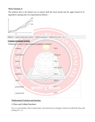
  • 9. Theta Notation, θ The notation θ(n) is the formal way to express both the lower bound and the upper bound of an algorithm's running time. It is represented as follows − θ(f(n)) = { g(n) if and only if g(n) = Ο(f(n)) and g(n) = Ω(f(n)) for all n > n0. } CommonAsymptoticNotations Following is a list of some common asymptotic notations − constant − Ο(1) logarithmic − Ο(log n) linear − Ο(n) n log n − Ο(n log n) quadratic − Ο(n2 ) cubic − Ο(n3 ) polynomial − nΟ(1) exponential − 2Ο(n) Mathematical Notation and function 1. Floor and Ceiling Functions: If x is a real number, then it means that x lies between two integers which are called the floor and ceiling of x. i.e.
  • 10. |_x_| is called the floor of x. It is the greatest integer that is not greater than x. | x | is called the ceiling of x. It is the smallest integer that is not less than x. If x is itself an integer, then |_x_| = | x |, otherwise |_x_| + 1 = | x | E.g. |_3.14_|=3,|_-8.5_|=-9,|_7_|=7 | 3.14 |= 4, | -8.5 | = -8, | 7 |= 7 2. Remainder Function (Modular Arithmetic): If k is any integer and M is a positive integer, then: k (mod M) gives the integer remainder when k is divided by M. E.g. 25(mod7)=4 25(mod 5) = 0 3. Integer and Absolute Value Functions: If x is a real number, then integer function INT(x) will convert x into integer and the fractional part is removed. E.g. INT(3.14)=3 INT (-8.5) = -8 The absolute function ABS(x) or | x | gives the absolute value of x i.e. it gives the positive value of x even if x is negative. E.g. ABS(-15)=15orABS|-15|=15 ABS(7)=7orABS7|=7 ABS(-3.33) = 3.33 or ABS | -3.33 | = 3.33 4. Summation Symbol (Sums): The symbol which is used to denote summation is a Greek letter Sigma ?. Let a1, a2, a3, ….. , an be a sequence of numbers. Then the sum a1 + a2 + a3 + ….. + an will be written as: n ? aj j=1 where j is called the dummy index or dummy variable. E.g. n ?j=1+2+3+…..+n j=1 5. Factorial Function: n! denotes the product of the positive integers from 1 to n. n! is read as ‘n factorial’, i.e. n! = 1 * 2 * 3 * ….. * (n-2) * (n-1) * n
  • 11. E.g. 4!=1*2*3*4=24 5! = 5 * 4! = 120 6. Permutations: Let we have a set of n elements. A permutation of this set means the arrangement of the elements of the set in some order. E.g. Suppose the set contains a, b and c. The various permutations of these elements can be: abc, acb, bac, bca, cab, cba. If there are n elements in the set then there will be n! permutations of those elements. It means if the set has 3 elements then there will be 3! = 1 * 2 * 3 = 6 permutations of the elements. 7. Exponents and Logarithms: Exponent means how many times a number is multiplied by itself. If m is a positive integer, then: am=a*a*a*…..*a(m times) and a-m=1/am E.g. 24=2*2*2*2=16 2-4 = 1 / 24 = 1 / 16 Control structures A control structure is a block of programming that analyzes variables and chooses a direction in which to go based on given parameters. The term flow control details the direction the program takes (which way program control "flows"). Hence it is the basic decision-making process in computing; flow control determines how a computer will respond when given certain conditions and parameters. Basic Terminologies Those initial conditions and parameters are called preconditions. Preconditions are the state of variables before entering a control structure. Based on those preconditions, the computer runs an algorithm (the control structure) to determine what to do. The result is called a post condition. Post conditions are the state of variables after the algorithm is run. An Example Let us analyze flow control by using traffic flow as a model. A vehicle is arriving at an intersection. Thus, the precondition is the vehicle is in motion. Suppose the traffic light at the intersection is red. The control structure must determine the proper course of action to assign to the vehicle. Precondition: The vehicle is in motion. Treatments of Information through Control Structures Is the traffic light green? If so, then the vehicle may stay in motion. Is the traffic light red? If so, then the vehicle must stop. End of Treatment
  • 12. Post condition: The vehicle comes to a stop. Thus, upon exiting the control structure, the vehicle is stopped. can also be form as a structure IF-THEN Statement[edit] The IF-THEN statement is a simple control that tests whether a condition is true or false. The condition can include a variable, or be a variable. If the variable is an integer 2, it will be true, because any number that is not zero will be true. If the condition is true, then an action occurs. If the condition is false, nothing is done. To illustrate: IF variable is true THEN take this course of action. If the variable indeed holds a value consistent with being true, then the course of action is taken. If the variable is not true, then there is no course of action taken. IF-THEN-ELSE Statement IF-THEN statements test for only one action. With an IF-THEN-ELSE statement, the control can "look both ways" so to speak, and take a secondary course of action. If the condition is true, then an action occurs. If the condition is false, take an alternate action. To illustrate: IF variable is true THEN take this course of action ELSE call another routine In this case, if the variable is true, it takes a certain course of action and completely skips the ELSE clause. If the variable is false, the control structure calls a routine and completely skips the THEN clause. Note that you can combine ELSE's with other IF's, allowing several tests to be made. In an IF- THEN-ELSEIF-THEN-ELSEIF-THEN-ELSEIF-THEN structure, tests will stop as soon as a condition is true. That's why you'd probably want to put the most "likely" test first, for efficiency (Remembering that ELSE's are skipped if the first condition is true, meaning that the remaining portions of the IF-THEN-ELSEIF... would not be processed). eg: In case your computer doesn't start IF a floppy disk is in the drive THEN remove it and restart ELSE IF you don't have any OS installed THEN install an OS ELSE call the hotline You can have as many ELSE IF's as you like. WHILE and DO-WHILE Loops A WHILE loop is a process in which a loop is initiated until a condition has been met. This structure is useful when performing iterative instructions to satisfy a certain parameter. To illustrate: Precondition: variable X is equal to 1 WHILE X is not equal to 9 Add 1 to X
  • 13. This routine will add 1 to X until X is equal to 9, at which point the control structure will quit and move on to the next instruction. Note that when the structure quits, it will not execute the Add function: when X is equal to 9, it will skip over the clause that is attached to the WHILE. This instruction is useful if a parameter needs to be tested repeatedly before acceptance. DO-WHILE Loops A DO-WHILE loop is nearly the exact opposite to a WHILE loop. A WHILE loop initially checks to see if the parameters have been satisfied before executing an instruction. A DO-WHILE loop executes the instruction before checking the parameters. To illustrate: DO Add 1 to X WHILE X is not equal 9 As you can see, the example differs from the first illustration, where the DO action is taken before the WHILE. The WHILE is inclusive in the DO. As such, if the WHILE results in a false (X is equal to 9), the control structure will break and will not perform another DO. Note that if X is equal to or greater than 9 prior to entering the DO-WHILE loop, then the loop will never terminate. FOR Loops A FOR loop is an extension of a while loop. A for loop usually has three commands. The first is used to set a starting point (like x = 0). The second is the end condition (same as in a while loop) and is run every round. The third is also run every round and is usually used to modify a value used in the condition block. FOR X is 0. X is less than 10. add 1 to X. This loop would be run 10 times (x being 0 to 9) so you won't have to think about the X variable in the loop you can just put code there. Here is a while loop that does the same: X is 0 WHILE X is less than 10 add 1 to X Some programming languages also have a foreach loop which will be useful when working with arrays (and collections). A foreach loop is an even more automated while loop that cycles through array's and such. Example : FOREACH student IN students give a good mark to student DataStructures&AlgorithmBasicConcepts DataDefinition Data Definition defines a particular data with the following characteristics. • Atomic − Definition should define a single concept. • Traceable − Definition should be able to be mapped to some data element. • Accurate − Definition should be unambiguous. • Clear and Concise − Definition should be understandable. DataObject Data Object represents an object having a data.
  • 14. DataType Data type is a way to classify various types of data such as integer, string, etc. which determines the values that can be used with the corresponding type of data, the type of operations that can be performed on the corresponding type of data. There are two data types − • Built-in Data Type • Derived Data Type Built-in Data Type Those data types for which a language has built-in support are known as Built-in Data types. For example, most of the languages provide the following built-in data types. • Integers • Boolean (true, false) • Floating (Decimal numbers) • Character and Strings Derived Data Type Those data types which are implementation independent as they can be implemented in one or the other way are known as derived data types. These data types are normally built by the combination of primary or built-in data types and associated operations on them. For example − • List • Array • Stack • Queue Reference https://keithlyons.me/blog/2018/11/07/el30-graphing/ https://www.tutorialspoint.com/data_structures_algorithms/index.htm https://www.geeksforgeeks.org/data-structures/