Mesh Processing Course : Geodesics
3 likes1,487 views

This document discusses geodesic data processing on Riemannian manifolds. It defines geodesic distances as the shortest path between two points on the manifold according to the Riemannian metric. Methods are presented for computing geodesic distances and curves, including iterative schemes and fast marching. Applications discussed include shape recognition using geodesic statistics and geodesic meshing.


![Parametric Surfaces
Parameterized surface: u ⇥ R2 ⇤ (u) ⇥ M.
u1 ⇥
u2 ⇥u1
⇥
⇥u2
Curve in parameter domain: t ⇥ [0, 1] ⇤ (t) ⇥ D.
4](https://image.slidesharecdn.com/course-mesh-geodesic-121213055935-phpapp01/85/Mesh-Processing-Course-Geodesics-5-320.jpg)
![Parametric Surfaces
Parameterized surface: u ⇥ R2 ⇤ (u) ⇥ M.
u1 ⇥
u2 ⇥u1
¯
¯ ⇥
⇥u2
Curve in parameter domain: t ⇥ [0, 1] ⇤ (t) ⇥ D.
def.
Geometric realization: ¯ (t) = ⇥( (t)) M.
4](https://image.slidesharecdn.com/course-mesh-geodesic-121213055935-phpapp01/85/Mesh-Processing-Course-Geodesics-6-320.jpg)
![Parametric Surfaces
Parameterized surface: u ⇥ R2 ⇤ (u) ⇥ M.
u1 ⇥
u2 ⇥u1
¯
¯ ⇥
⇥u2
Curve in parameter domain: t ⇥ [0, 1] ⇤ (t) ⇥ D.
def.
Geometric realization: ¯ (t) = ⇥( (t)) M.
For an embedded manifold M Rn : ⇥
⇥ ⇥
First fundamental form: I = , ⇥ .
⇥ui ⇥uj i,j=1,2
Length of a curve
1 1 ⇥
def.
L( ) = ||¯ (t)||dt = (t)I (t) (t)dt.
0 0 4](https://image.slidesharecdn.com/course-mesh-geodesic-121213055935-phpapp01/85/Mesh-Processing-Course-Geodesics-7-320.jpg)


![Riemannian Manifold
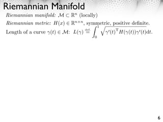
Riemannian manifold: M Rn (locally)
Riemannian metric: H(x) Rn , symmetric, positive definite.
n
1⇥
def. T
Length of a curve (t) M: L( ) = (t) H( (t)) (t)dt.
0
Euclidean space: M = Rn , H(x) = Idn .
2-D shape: M R2 , H(x) = Id2 .
Isotropic metric: H(x) = W (x)2 Idn .
Image processing: image I, W (x)2 = ( + || I(x)||) 1
.
Parametric surface: H(x) = Ix (1st fundamental form).
DTI imaging: M = [0, 1]3 , H(x)=di usion tensor.
W (x)
6](https://image.slidesharecdn.com/course-mesh-geodesic-121213055935-phpapp01/85/Mesh-Processing-Course-Geodesics-16-320.jpg)


![Anisotropy and Geodesics
Tensor eigen-decomposition:
T T
H(x) = 1 (x)e1 (x)e1 (x) + 2 (x)e2 (x)e2 (x) with 0 < 1 2,
{ H(x) 1}
4 ECCV-08 submission ID 1057
e2 (x)
2 (x)
1
2 x e1 (x)
Figure 2 shows examples of geodesic curves computed from a single starting
1
point (x)
MS = {x1 } in the center of the image = [0,11]2 and a set of points on the
2
boundary of . The geodesics are computed for a metric H(x) whose anisotropy
⇥(x) (defined in equation (2)) is to follow e1 (x).making the Riemannian space
Geodesics tend increasing, thus
progressively closer to the Euclidean space. ⇥1 (x) ⇥2 (x)
Local anisotropy of the metric: (x) = [0, 1]
⇥1 (x) + ⇥2 (x)
Image f
Image f = .1
= .95 = .2
= .7 = .5
= .5 = 10
= 8](https://image.slidesharecdn.com/course-mesh-geodesic-121213055935-phpapp01/85/Mesh-Processing-Course-Geodesics-25-320.jpg)


![Discretization Errors
For a mesh with N points: U [N ] RN solution of (U [N ] ) = U [N ]
Continuous geodesic distance U (x).
Linear interpolation: ˜
U [N ] (x) =
[N ]
Ui i (x)
i
Uniform convergence: ˜
||U [N ] U ||
N +
⇥ 0
20](https://image.slidesharecdn.com/course-mesh-geodesic-121213055935-phpapp01/85/Mesh-Processing-Course-Geodesics-53-320.jpg)
![Discretization Errors
For a mesh with N points: U [N ] RN solution of (U [N ] ) = U [N ]
Continuous geodesic distance U (x).
Linear interpolation: ˜
U [N ] (x) =
[N ]
Ui i (x)
i
Uniform convergence: ˜
||U [N ] U ||
N +
⇥ 0
1
Numerical evaluation: |UiN U (xi )|2
N i
20](https://image.slidesharecdn.com/course-mesh-geodesic-121213055935-phpapp01/85/Mesh-Processing-Course-Geodesics-54-320.jpg)


![Bending Invariant Recognition
Shape articulations:
[Zoopraxiscope, 1876]
29](https://image.slidesharecdn.com/course-mesh-geodesic-121213055935-phpapp01/85/Mesh-Processing-Course-Geodesics-65-320.jpg)
![Bending Invariant Recognition
Shape articulations:
[Zoopraxiscope, 1876]
Surface bendings:
˜
x1
˜
x2
M
[Elad, Kimmel, 2003]. [Bronstein et al., 2005].
29](https://image.slidesharecdn.com/course-mesh-geodesic-121213055935-phpapp01/85/Mesh-Processing-Course-Geodesics-66-320.jpg)


![Benging Invariant 2D Database
[Ling & Jacobs, PAMI 2007]
Our method
(min,med,max)
100 1D
100
4D
Average Precision
80
max only 80
Average Recall
60 [Ion et al. 2008] 60
40 40
20 1D 20
4D
0 0
0 10 20 30 40 0 20 40 60 80 100
Image Rank Average Recall
State of the art retrieval rates on this database.
32](https://image.slidesharecdn.com/course-mesh-geodesic-121213055935-phpapp01/85/Mesh-Processing-Course-Geodesics-71-320.jpg)


![Geodesic Sampling
Sampling {xi }i I of a manifold.
Farthest point algorithm: [Peyr´, Cohen, 2006]
e
xk+1 = argmax min d(xi , x)
x 0 i k
Metric Sampling](https://image.slidesharecdn.com/course-mesh-geodesic-121213055935-phpapp01/85/Mesh-Processing-Course-Geodesics-79-320.jpg)
![Geodesic Sampling
Sampling {xi }i I of a manifold.
Farthest point algorithm: [Peyr´, Cohen, 2006]
e
xk+1 = argmax min d(xi , x)
x 0 i k
Geodesic Voronoi: Metric Sampling
Ci = {x ⇥ j = i, d(xi , x) d(xj , x)}
Voronoi](https://image.slidesharecdn.com/course-mesh-geodesic-121213055935-phpapp01/85/Mesh-Processing-Course-Geodesics-80-320.jpg)
![Geodesic Sampling
Sampling {xi }i I of a manifold.
Farthest point algorithm: [Peyr´, Cohen, 2006]
e
xk+1 = argmax min d(xi , x)
x 0 i k
Geodesic Voronoi: Metric Sampling
Ci = {x ⇥ j = i, d(xi , x) d(xj , x)}
Geodesic Delaunay connectivity:
(xi xj ) ⇥ (Ci ⇧ Cj ⇤= ⌅)
geodesic Delaunay refinement. Voronoi Delaunay
distance conforming. triangulation conforming if the metric is “gradded”.](https://image.slidesharecdn.com/course-mesh-geodesic-121213055935-phpapp01/85/Mesh-Processing-Course-Geodesics-81-320.jpg)


![Approximation Driven Meshing
Linear approximation fM with M linear elements.
Minimize approximation error ||f fM ||Lp .
L optimal metrics for smooth functions:
Images: T (x) = |H(x)| (Hessian)
Surfaces: T (x) = |C(x)| (curvature tensor)
Isotropic Anisotropic
For edges and textures: use structure tensor.
[Peyr´ et al, 2008]
e
Anisotropic triangulation JPEG2000](https://image.slidesharecdn.com/course-mesh-geodesic-121213055935-phpapp01/85/Mesh-Processing-Course-Geodesics-86-320.jpg)
![Approximation Driven Meshing
Linear approximation fM with M linear elements.
Minimize approximation error ||f fM ||Lp .
L optimal metrics for smooth functions:
Images: T (x) = |H(x)| (Hessian)
Surfaces: T (x) = |C(x)| (curvature tensor)
Isotropic Anisotropic
For edges and textures: use structure tensor.
[Peyr´ et al, 2008]
e
Anisotropic triangulation JPEG2000
extension to handle
boundary approximation.
[Peyr´ et al, 2008]
e](https://image.slidesharecdn.com/course-mesh-geodesic-121213055935-phpapp01/85/Mesh-Processing-Course-Geodesics-87-320.jpg)


Mesh Processing Course : Geodesics
- 1. Geodesic Data Processing www.numerical-tours.com Gabriel Peyré CEREMADE, Université Paris-Dauphine
- 2. Local vs. Global Processing Local Processing Global Processing Differential Computations Geodesic Computations Surface filtering Front Propagation on Meshes Fourier on Meshes Surface Remeshing 2
- 3. Overview • Metrics and Riemannian Surfaces. • Geodesic Computation - Iterative Scheme • Geodesic Computation - Fast Marching • Shape Recognition with Geodesic Statistics • Geodesic Meshing 3
- 4. Parametric Surfaces Parameterized surface: u ⇥ R2 ⇤ (u) ⇥ M. u1 ⇥ u2 ⇥u1 ⇥ ⇥u2 4
- 5. Parametric Surfaces Parameterized surface: u ⇥ R2 ⇤ (u) ⇥ M. u1 ⇥ u2 ⇥u1 ⇥ ⇥u2 Curve in parameter domain: t ⇥ [0, 1] ⇤ (t) ⇥ D. 4
- 6. Parametric Surfaces Parameterized surface: u ⇥ R2 ⇤ (u) ⇥ M. u1 ⇥ u2 ⇥u1 ¯ ¯ ⇥ ⇥u2 Curve in parameter domain: t ⇥ [0, 1] ⇤ (t) ⇥ D. def. Geometric realization: ¯ (t) = ⇥( (t)) M. 4
- 7. Parametric Surfaces Parameterized surface: u ⇥ R2 ⇤ (u) ⇥ M. u1 ⇥ u2 ⇥u1 ¯ ¯ ⇥ ⇥u2 Curve in parameter domain: t ⇥ [0, 1] ⇤ (t) ⇥ D. def. Geometric realization: ¯ (t) = ⇥( (t)) M. For an embedded manifold M Rn : ⇥ ⇥ ⇥ First fundamental form: I = , ⇥ . ⇥ui ⇥uj i,j=1,2 Length of a curve 1 1 ⇥ def. L( ) = ||¯ (t)||dt = (t)I (t) (t)dt. 0 0 4
- 8. Isometric and Conformal Surface not homeomorphic to a disk: M is locally isometric to the plane: I = Id. Exemple: M =cylinder.
- 9. Isometric and Conformal Surface not homeomorphic to a disk: M is locally isometric to the plane: I = Id. Exemple: M =cylinder. ⇥ is conformal: I (u) = (u)Id. Exemple: stereographic mapping plane sphere.
- 10. Riemannian Manifold Riemannian manifold: M Rn (locally) Riemannian metric: H(x) Rn , symmetric, positive definite. n 1⇥ def. T Length of a curve (t) M: L( ) = (t) H( (t)) (t)dt. 0 6
- 11. Riemannian Manifold Riemannian manifold: M Rn (locally) Riemannian metric: H(x) Rn , symmetric, positive definite. n 1⇥ def. T Length of a curve (t) M: L( ) = (t) H( (t)) (t)dt. 0 Euclidean space: M = Rn , H(x) = Idn . W (x) 6
- 12. Riemannian Manifold Riemannian manifold: M Rn (locally) Riemannian metric: H(x) Rn , symmetric, positive definite. n 1⇥ def. T Length of a curve (t) M: L( ) = (t) H( (t)) (t)dt. 0 Euclidean space: M = Rn , H(x) = Idn . 2-D shape: M R2 , H(x) = Id2 . W (x) 6
- 13. Riemannian Manifold Riemannian manifold: M Rn (locally) Riemannian metric: H(x) Rn , symmetric, positive definite. n 1⇥ def. T Length of a curve (t) M: L( ) = (t) H( (t)) (t)dt. 0 Euclidean space: M = Rn , H(x) = Idn . 2-D shape: M R2 , H(x) = Id2 . Isotropic metric: H(x) = W (x)2 Idn . W (x) 6
- 14. Riemannian Manifold Riemannian manifold: M Rn (locally) Riemannian metric: H(x) Rn , symmetric, positive definite. n 1⇥ def. T Length of a curve (t) M: L( ) = (t) H( (t)) (t)dt. 0 Euclidean space: M = Rn , H(x) = Idn . 2-D shape: M R2 , H(x) = Id2 . Isotropic metric: H(x) = W (x)2 Idn . Image processing: image I, W (x)2 = ( + || I(x)||) 1 . W (x) 6
- 15. Riemannian Manifold Riemannian manifold: M Rn (locally) Riemannian metric: H(x) Rn , symmetric, positive definite. n 1⇥ def. T Length of a curve (t) M: L( ) = (t) H( (t)) (t)dt. 0 Euclidean space: M = Rn , H(x) = Idn . 2-D shape: M R2 , H(x) = Id2 . Isotropic metric: H(x) = W (x)2 Idn . Image processing: image I, W (x)2 = ( + || I(x)||) 1 . Parametric surface: H(x) = Ix (1st fundamental form). W (x) 6
- 16. Riemannian Manifold Riemannian manifold: M Rn (locally) Riemannian metric: H(x) Rn , symmetric, positive definite. n 1⇥ def. T Length of a curve (t) M: L( ) = (t) H( (t)) (t)dt. 0 Euclidean space: M = Rn , H(x) = Idn . 2-D shape: M R2 , H(x) = Id2 . Isotropic metric: H(x) = W (x)2 Idn . Image processing: image I, W (x)2 = ( + || I(x)||) 1 . Parametric surface: H(x) = Ix (1st fundamental form). DTI imaging: M = [0, 1]3 , H(x)=di usion tensor. W (x) 6
- 17. Geodesic Distances Geodesic distance metric over M Rn dM (x, y) = min L( ) (0)=x, (1)=y Geodesic curve: (t) such that L( ) = dM (x, y). def. Distance map to a starting point x0 M: Ux0 (x) = dM (x0 , x). 7
- 18. Geodesic Distances Geodesic distance metric over M Rn dM (x, y) = min L( ) (0)=x, (1)=y Geodesic curve: (t) such that L( ) = dM (x, y). def. Distance map to a starting point x0 M: Ux0 (x) = dM (x0 , x). metric geodesics Euclidean 7
- 19. Geodesic Distances Geodesic distance metric over M Rn dM (x, y) = min L( ) (0)=x, (1)=y Geodesic curve: (t) such that L( ) = dM (x, y). def. Distance map to a starting point x0 M: Ux0 (x) = dM (x0 , x). metric geodesics Euclidean Shape 7
- 20. Geodesic Distances Geodesic distance metric over M Rn dM (x, y) = min L( ) (0)=x, (1)=y Geodesic curve: (t) such that L( ) = dM (x, y). def. Distance map to a starting point x0 M: Ux0 (x) = dM (x0 , x). metric geodesics Euclidean Shape Isotropic 7
- 21. Geodesic Distances Geodesic distance metric over M Rn dM (x, y) = min L( ) (0)=x, (1)=y Geodesic curve: (t) such that L( ) = dM (x, y). def. Distance map to a starting point x0 M: Ux0 (x) = dM (x0 , x). metric geodesics Euclidean Shape Isotropic Anisotropic 7
- 22. Geodesic Distances Geodesic distance metric over M Rn dM (x, y) = min L( ) (0)=x, (1)=y Geodesic curve: (t) such that L( ) = dM (x, y). def. Distance map to a starting point x0 M: Ux0 (x) = dM (x0 , x). metric geodesics Euclidean Shape Isotropic Anisotropic Surface 7
- 23. Anisotropy and Geodesics Tensor eigen-decomposition: T T H(x) = 1 (x)e1 (x)e1 (x) + 2 (x)e2 (x)e2 (x) with 0 < 1 2, { H(x) 1} e2 (x) 2 (x) 1 2 x e1 (x) 1 M 1 (x) 2 8
- 24. Anisotropy and Geodesics Tensor eigen-decomposition: T T H(x) = 1 (x)e1 (x)e1 (x) + 2 (x)e2 (x)e2 (x) with 0 < 1 2, { H(x) 1} e2 (x) 2 (x) 1 2 x e1 (x) 1 M 1 (x) 2 Geodesics tend to follow e1 (x). 8
- 25. Anisotropy and Geodesics Tensor eigen-decomposition: T T H(x) = 1 (x)e1 (x)e1 (x) + 2 (x)e2 (x)e2 (x) with 0 < 1 2, { H(x) 1} 4 ECCV-08 submission ID 1057 e2 (x) 2 (x) 1 2 x e1 (x) Figure 2 shows examples of geodesic curves computed from a single starting 1 point (x) MS = {x1 } in the center of the image = [0,11]2 and a set of points on the 2 boundary of . The geodesics are computed for a metric H(x) whose anisotropy ⇥(x) (defined in equation (2)) is to follow e1 (x).making the Riemannian space Geodesics tend increasing, thus progressively closer to the Euclidean space. ⇥1 (x) ⇥2 (x) Local anisotropy of the metric: (x) = [0, 1] ⇥1 (x) + ⇥2 (x) Image f Image f = .1 = .95 = .2 = .7 = .5 = .5 = 10 = 8
- 26. Isotropic Metric Design Image-based potential: H(x) = W (x)2 Id2 , W (x) = ( + |f (x) c|) Image f Metric W (x) Distance Ux0 (x) Geodesic curve (t) 9
- 27. Isotropic Metric Design Image-based potential: H(x) = W (x)2 Id2 , W (x) = ( + |f (x) c|) Image f Metric W (x) Distance Ux0 (x) Geodesic curve (t) Gradient-based potential: W (x) = ( + || x f ||) Image f Metric W (x) U{x0 ,x1 } Geodesics 9
- 28. Isotropic Metric Design: Vessels ˜ Remove background: f = G ⇥ f f, ⇥vessel width. f ˜ f ˜ W = ( + max(f , 0)) 10
- 29. Isotropic Metric Design: Vessels ˜ Remove background: f = G ⇥ f f, ⇥vessel width. f ˜ f ˜ W = ( + max(f , 0)) 3D Volumetric datasets: 10
- 30. Overview • Metrics and Riemannian Surfaces. • Geodesic Computation - Iterative Scheme • Geodesic Computation - Fast Marching • Shape Recognition with Geodesic Statistics • Geodesic Meshing 11
- 31. Eikonal Equation and Viscosity Solution Distance map: U (x) = d(x0 , x) Theorem: U is the unique viscosity solution of || U (x)||H(x) 1 = 1 with U (x0 ) = 0 where ||v||A = v Av 12
- 32. Eikonal Equation and Viscosity Solution Distance map: U (x) = d(x0 , x) Theorem: U is the unique viscosity solution of || U (x)||H(x) 1 = 1 with U (x0 ) = 0 where ||v||A = v Av Geodesic curve between x1 and x0 solves (0) = x1 (t) = ⇥t H( (t)) 1 Ux0 ( (t)) with t >0 12
- 33. Eikonal Equation and Viscosity Solution Distance map: U (x) = d(x0 , x) Theorem: U is the unique viscosity solution of || U (x)||H(x) 1 = 1 with U (x0 ) = 0 where ||v||A = v Av Geodesic curve between x1 and x0 solves (0) = x1 (t) = ⇥t H( (t)) 1 Ux0 ( (t)) with t >0 Example: isotropic metric H(x) = W (x)2 Idn , || U (x)|| = W (x) and (t) = ⇥t U ( (t)) 12
- 34. Simplified Proof 1 U (x) = min L( ) = 0 H( (t)) (t), (t) dt :x0 x ||⇤V (x)||2 1 = H 1 (x)⇤V (x), ⇤V (x)⇥ = 1, V solving H V (x0 ) = 0.
- 35. Simplified Proof 1 U (x) = min L( ) = 0 H( (t)) (t), (t) dt :x0 x ||⇤V (x)||2 1 = H 1 (x)⇤V (x), ⇤V (x)⇥ = 1, V solving H V (x0 ) = 0. U V Let : x0 x be any smooth curve. If V is smooth on : C.S. , ⇤V ⇥ = H 1/2 , H 1/2 ⇤V ⇥ ||H 1/2 ||||H 1/2 ⇤V || =1
- 36. Simplified Proof 1 U (x) = min L( ) = 0 H( (t)) (t), (t) dt :x0 x ||⇤V (x)||2 1 = H 1 (x)⇤V (x), ⇤V (x)⇥ = 1, V solving H V (x0 ) = 0. U V Let : x0 x be any smooth curve. If V is smooth on : C.S. , ⇤V ⇥ = H 1/2 , H 1/2 ⇤V ⇥ ||H 1/2 ||||H 1/2 ⇤V || =1 1 1 L( ) = 0 ||H 1/2 || 0 ⇥ , ⌅V ⇤ = V ( (1)) V ( (0)) = V (x) =0 = U (x) = min L( ) V (x)
- 37. Simplified Proof (cont.) U V Let x be arbitrary. Define: (t) = H 1 ( (t)) V ( (t)) (0) = x x x0
- 38. Simplified Proof (cont.) U V Let x be arbitrary. Define: (t) = H 1 ( (t)) V ( (t)) (0) = x x If V is smooth on ([0, tmax )), then dV ( (t)) = (t), V ( (t)) = 1 dt x0 = (tmax ) = x0
- 39. Simplified Proof (cont.) U V Let x be arbitrary. Define: (t) = H 1 ( (t)) V ( (t)) (0) = x x If V is smooth on ([0, tmax )), then dV ( (t)) = (t), V ( (t)) = 1 dt x0 = (tmax ) = x0 One has: H , = H V, V = 1 1 =1 tmax tmax U (x) L( ) = 0 H , = 0 H , tmax = 0 , V = V ( (tmax )) + V ( (0)) = V (x) =0 13 14
- 40. Discretization x0 Control (derivative-free) formulation: B(x) y U (x) = d(x0 , x) is the unique solution of U (x) = (U )(x) = min U (y) + d(x, y) x y B(x) 15
- 41. Discretization x0 Control (derivative-free) formulation: B(x) y U (x) = d(x0 , x) is the unique solution of U (x) = (U )(x) = min U (y) + d(x, y) x y B(x) Manifold discretization: triangular mesh. U discretization: linear finite elements. B(x) H discretization: constant on each triangle. xi xk xj 15
- 42. Discretization x0 Control (derivative-free) formulation: B(x) y U (x) = d(x0 , x) is the unique solution of U (x) = (U )(x) = min U (y) + d(x, y) x y B(x) Manifold discretization: triangular mesh. U discretization: linear finite elements. B(x) H discretization: constant on each triangle. xi xk Ui = (U )i = min Vi,j,k f =(i,j,k) xj Vi,j,k = min tUj + (1 t)Uk xi 0 t 1 xk +||txj + (1 t)xk xi ||Hijk explicit solution (solving quadratic equation). txj + (1 t)xk on regular grid: equivalent to upwind FD. xj 15
- 43. Update Step on a triangulation (U )i = min Vi,j,k f =(i,j,k) Discrete Eikonal equation: Vi,j,k = min tUj + (1 t)Uk +||txj + (1 t)xk xi ||Hijk 0 t 1 xi xk xj 16
- 44. Update Step on a triangulation (U )i = min Vi,j,k f =(i,j,k) Discrete Eikonal equation: Vi,j,k = min tUj + (1 t)Uk +||txj + (1 t)xk xi ||Hijk 0 t 1 Distance function in (i, j, k): U (x) = x xi , g + d Unknowns: gradient = Vi,j,k xi xk xj g 16
- 45. Update Step on a triangulation (U )i = min Vi,j,k f =(i,j,k) Discrete Eikonal equation: Vi,j,k = min tUj + (1 t)Uk +||txj + (1 t)xk xi ||Hijk 0 t 1 Distance function in (i, j, k): U (x) = x xi , g + d Unknowns: gradient = Vi,j,k Notations: Hi,j,k = w2 Id3 (for simplifity) xi X = (xj xi , xk xi ) R d 2 xk u = (Uj , Uk ) R2 I = (1, 1) R2 xj g S = (X X) 1 R 2 2 16
- 46. Update Step on a triangulation (cont.) Find g = X , R2 and d = Vi,j,k . xi X g + dI = u = = S(u dI) xk xj 0 17
- 47. Update Step on a triangulation (cont.) Find g = X , R2 and d = Vi,j,k . xi X g + dI = u = = S(u dI) xk Discrete Eikonal equation: || U (xi )|| = ||g|| = w xj 0 17
- 48. Update Step on a triangulation (cont.) Find g = X , R2 and d = Vi,j,k . xi X g + dI = u = = S(u dI) xk Discrete Eikonal equation: || U (xi )|| = ||g|| = w xj 0 Quadratic equation: a = SI, I ||XS(u dI)||2 = w2 b = SI, u = c = Su, u w2 d 2 2bd + c = 0 17
- 49. Update Step on a triangulation (cont.) Find g = X , R2 and d = Vi,j,k . xi 0 X g + dI = u = = S(u dI) 1 xk Discrete Eikonal equation: || U (xi )|| = ||g|| = w xj 0 Quadratic equation: a = SI, I ||XS(u dI)||2 = w2 b = SI, u = c = Su, u w2 d 2 2bd + c = 0 b+ Admissible solution: d= = b2 ac a d if 0 dj = Uj + Wi ||xi xj || (ui ) = min(dj , dk ) otherwise. 17
- 50. Numerical Schemes Fixed point equation: U = (U ) is monotone: U V = (U ) (V ) Iterative schemes: U (0) = 0, U ( +1) = (U ( ) ) || (U ( ) ) U ( ) || = U( +1) U( ) C<+ U( ) U solving (U ) = U U( ) 18
- 51. Numerical Schemes Fixed point equation: U = (U ) is monotone: U V = (U ) (V ) Iterative schemes: U (0) = 0, U ( +1) = (U ( ) ) || (U ( ) ) U ( ) || = U( +1) U( ) C<+ U( ) U solving (U ) = U Minimal path extraction: ( +1) = ( ) ⇥ H( ( ) ) 1 U( ( ) ) U( ) 18
- 52. Numerical Examples on Meshes 19
- 53. Discretization Errors For a mesh with N points: U [N ] RN solution of (U [N ] ) = U [N ] Continuous geodesic distance U (x). Linear interpolation: ˜ U [N ] (x) = [N ] Ui i (x) i Uniform convergence: ˜ ||U [N ] U || N + ⇥ 0 20
- 54. Discretization Errors For a mesh with N points: U [N ] RN solution of (U [N ] ) = U [N ] Continuous geodesic distance U (x). Linear interpolation: ˜ U [N ] (x) = [N ] Ui i (x) i Uniform convergence: ˜ ||U [N ] U || N + ⇥ 0 1 Numerical evaluation: |UiN U (xi )|2 N i 20
- 55. Overview • Metrics and Riemannian Surfaces. • Geodesic Computation - Iterative Scheme • Geodesic Computation - Fast Marching • Shape Recognition with Geodesic Statistics • Geodesic Meshing 21
- 56. Causal Updates Causality condition: j i, (U )i Uj The value of Ui depends on {Uj }j with Uj Ui . Compute (U )i using an optimal ordering. Front propagation, O(N log(N )) operations. 22
- 57. Causal Updates Causality condition: j i, (U )i Uj xi,j+1 The value of Ui depends on {Uj }j with Uj Ui . Compute (U )i using an optimal ordering. xi,j xi+1,j Front propagation, O(N log(N )) operations. Isotropic H(x) = W (x)2 Id, square grid. u = (U )i is the solution of max(u Ui 1,j , u Ui+1,j , 0)2 + max(u Ui,j 1, u Ui,j+1 , 0)2 = h2 Wi,j 2 (upwind derivatives) 22
- 58. Causal Updates Causality condition: j i, (U )i Uj xi,j+1 The value of Ui depends on {Uj }j with Uj Ui . Compute (U )i using an optimal ordering. xi,j xi+1,j Front propagation, O(N log(N )) operations. Isotropic H(x) = W (x)2 Id, square grid. u = (U )i is the solution of Good max(u Ui 1,j , u Ui+1,j , 0)2 + max(u Ui,j 1, u Ui,j+1 , 0)2 = h2 Wi,j 2 xi Bad xk (upwind derivatives) xj Surface (first fundamental form) triangulation with no obtuse angles. Bad Good 22
- 59. Front Propagation Front Ft , Ft = {i Ui t} Ft x0 State Si {Computed, F ront, F ar} Algorithm: Far Front Computed. 1) Select front point with minimum Ui Iteration 2) Move from Front to Computed . 3) Update Uj = (U )j for neighbors and 23
- 60. Fast Marching on an Image 24
- 61. Fast Marching on Shapes and Surfaces 25
- 62. Volumetric Datasets 26
- 63. Propagation in 3D 27
- 64. Overview • Metrics and Riemannian Surfaces. • Geodesic Computation - Iterative Scheme • Geodesic Computation - Fast Marching • Shape Recognition with Geodesic Statistics • Geodesic Meshing 28
- 65. Bending Invariant Recognition Shape articulations: [Zoopraxiscope, 1876] 29
- 66. Bending Invariant Recognition Shape articulations: [Zoopraxiscope, 1876] Surface bendings: ˜ x1 ˜ x2 M [Elad, Kimmel, 2003]. [Bronstein et al., 2005]. 29
- 67. 2D Shapes 2D shape: connected, closed compact set S R2 . Piecewise-smooth boundary S. Geodesic distance in S for uniform metric: 1 def. def. dS (x, y) = min L( ) where L( ) = | (t)|dt, ⇥P(x,y) 0 Shape S Geodesics 30
- 68. Distribution of Geodesic Distances Distribution of distances 80 60 to a point x: {dM (x, y)}y 40 M 20 0 80 60 40 20 0 80 60 40 20 0 31
- 69. Distribution of Geodesic Distances Distribution of distances 80 60 to a point x: {dM (x, y)}y 40 M 20 0 80 60 Extract a statistical measure 40 20 0 a0 (x) = min dM (x, y). 80 60 40 y 20 0 a1 (x) = median dM (x, y). y a2 (x) = max dM (x, y). y x x x Min Median Max 31
- 70. Distribution of Geodesic Distances Distribution of distances 80 60 to a point x: {dM (x, y)}y 40 M 20 0 80 60 Extract a statistical measure 40 20 0 a0 (x) = min dM (x, y). 80 60 40 y 20 0 a1 (x) = median dM (x, y). y a2 (x) = max dM (x, y). a2 y a(x) x x x a1 a0 Min Median Max 31
- 71. Benging Invariant 2D Database [Ling & Jacobs, PAMI 2007] Our method (min,med,max) 100 1D 100 4D Average Precision 80 max only 80 Average Recall 60 [Ion et al. 2008] 60 40 40 20 1D 20 4D 0 0 0 10 20 30 40 0 20 40 60 80 100 Image Rank Average Recall State of the art retrieval rates on this database. 32
- 72. Perspective: Textured Shapes Take into account a texture f (x) on the shape. Compute a saliency field W (x), e.g. edge detector. 1 def. Compute weighted curve lengths: L( ) = W ( (t))|| (t)||dt. 0 Euclidean Image f (x) Weighted || f (x)|| Max Min 33
- 73. Overview • Metrics and Riemannian Surfaces. • Geodesic Computation - Iterative Scheme • Geodesic Computation - Fast Marching • Shape Recognition with Geodesic Statistics • Geodesic Meshing 34
- 74. Meshing Images, Shapes and Surfaces Vertices V = {vi }M . Triangulation (V, F): i=1 Faces F {1, . . . , M }3 . M Image approximation: fM = m ⇥m m=1 = argmin ||f µm ⇥m || µ m ⇥m (vi ) = m i is a ne on each face of F. 35
- 75. Meshing Images, Shapes and Surfaces Vertices V = {vi }M . Triangulation (V, F): i=1 Faces F {1, . . . , M }3 . M Image approximation: fM = m ⇥m m=1 = argmin ||f µm ⇥m || µ m ⇥m (vi ) = m i is a ne on each face of F. There exists (V, F) such that ||f fM || Cf M 2 Optimal (V, F): NP-hard. 35
- 76. Meshing Images, Shapes and Surfaces Vertices V = {vi }M . Triangulation (V, F): i=1 Faces F {1, . . . , M }3 . M Image approximation: fM = m ⇥m m=1 = argmin ||f µm ⇥m || µ m ⇥m (vi ) = m i is a ne on each face of F. There exists (V, F) such that ||f fM || Cf M 2 Optimal (V, F): NP-hard. Domain meshing: Conforming to complicated boundary. Capturing PDE solutions: Boundary layers, chocs . . . 35
- 77. Riemannian Sizing Field Sampling {xi }i I of a manifold. Distance conforming: ⇤ xi ⇥ xj , d(xi , xj ) e1 (x) 1 1 (x) 2 e2 (x) Triangulation conforming: x ⇥ =( xi ⇤ xj ⇤ xk ) ⇥ x ||x x ||T (x ) 2 (x) 1 2 Building triangulation ⇥ Ellipsoid packing ⇥ Global integration of local sizing field 36
- 78. Geodesic Sampling Sampling {xi }i I of a manifold. Metric Sampling
- 79. Geodesic Sampling Sampling {xi }i I of a manifold. Farthest point algorithm: [Peyr´, Cohen, 2006] e xk+1 = argmax min d(xi , x) x 0 i k Metric Sampling
- 80. Geodesic Sampling Sampling {xi }i I of a manifold. Farthest point algorithm: [Peyr´, Cohen, 2006] e xk+1 = argmax min d(xi , x) x 0 i k Geodesic Voronoi: Metric Sampling Ci = {x ⇥ j = i, d(xi , x) d(xj , x)} Voronoi
- 81. Geodesic Sampling Sampling {xi }i I of a manifold. Farthest point algorithm: [Peyr´, Cohen, 2006] e xk+1 = argmax min d(xi , x) x 0 i k Geodesic Voronoi: Metric Sampling Ci = {x ⇥ j = i, d(xi , x) d(xj , x)} Geodesic Delaunay connectivity: (xi xj ) ⇥ (Ci ⇧ Cj ⇤= ⌅) geodesic Delaunay refinement. Voronoi Delaunay distance conforming. triangulation conforming if the metric is “gradded”.
- 82. Adaptive Meshing # samples
- 83. Adaptive Meshing # samples Texture Metric Uniform Adaptive
- 84. Approximation Driven Meshing Linear approximation fM with M linear elements. Minimize approximation error ||f fM ||Lp . Isotropic
- 85. Approximation Driven Meshing Linear approximation fM with M linear elements. Minimize approximation error ||f fM ||Lp . L optimal metrics for smooth functions: Images: T (x) = |H(x)| (Hessian) Surfaces: T (x) = |C(x)| (curvature tensor) Isotropic Anisotropic
- 86. Approximation Driven Meshing Linear approximation fM with M linear elements. Minimize approximation error ||f fM ||Lp . L optimal metrics for smooth functions: Images: T (x) = |H(x)| (Hessian) Surfaces: T (x) = |C(x)| (curvature tensor) Isotropic Anisotropic For edges and textures: use structure tensor. [Peyr´ et al, 2008] e Anisotropic triangulation JPEG2000
- 87. Approximation Driven Meshing Linear approximation fM with M linear elements. Minimize approximation error ||f fM ||Lp . L optimal metrics for smooth functions: Images: T (x) = |H(x)| (Hessian) Surfaces: T (x) = |C(x)| (curvature tensor) Isotropic Anisotropic For edges and textures: use structure tensor. [Peyr´ et al, 2008] e Anisotropic triangulation JPEG2000 extension to handle boundary approximation. [Peyr´ et al, 2008] e
- 88. Conclusion Riemannian tensors encode geometric features. Size, orientation, anisotropy. Computing geodesic distance: iterative vs. propagation. 40
- 89. Conclusion Riemannian tensors encode geometric features. Size, orientation, anisotropy. Computing geodesic distance: iterative vs. propagation. Using geodesic curves: image segmentation. Using geodesic distance: image and surface meshing 40