Signal Processing Course : Sparse Regularization of Inverse Problems
3 likes•3,932 views

The document discusses sparse regularization for inverse problems. It describes how sparse regularization can be used for tasks like denoising, inpainting, and image separation by posing them as optimization problems that minimize data fidelity and an L1 sparsity prior on the coefficients. Iterative soft thresholding is presented as an algorithm for solving the noisy sparse regularization problem. Examples are given of how sparse wavelet regularization can outperform other regularizers like Sobolev for tasks like image deblurring.


![Noiseless Sparse Regularization
Noiseless measurements: y = x0
x
x
x= x=
y y
x argmin |xm | x argmin |xm |2
x=y m x=y m
Convex linear program.
Interior points, cf. [Chen, Donoho, Saunders] “basis pursuit”.
Douglas-Rachford splitting, see [Combettes, Pesquet].](https://image.slidesharecdn.com/course-signal-inverse-pbm-sparse-121213053017-phpapp01/85/Signal-Processing-Course-Sparse-Regularization-of-Inverse-Problems-37-320.jpg)


![Noisy Sparse Regularization
Noisy measurements: y = x0 + w
1
x argmin ||y x||2 + ||x||1
x RQ 2 Equivalence
Data fidelity Regularization
x argmin ||x||1
|| x y||
|
x=
Algorithms: x y|
Iterative soft thresholding
Forward-backward splitting
see [Daubechies et al], [Pesquet et al], etc
Nesterov multi-steps schemes.](https://image.slidesharecdn.com/course-signal-inverse-pbm-sparse-121213053017-phpapp01/85/Signal-Processing-Course-Sparse-Regularization-of-Inverse-Problems-40-320.jpg)


![Image Separation
Model: f = f1 + f2 + w, (f1 , f2 ) components, w noise.
Union dictionary: =[ 1, 2] RQ (N1 +N2 )
Recovered component: fi = i xi .
1
(x1 , x2 ) argmin ||f x||2 + ||x||1
x=(x1 ,x2 ) RN 2](https://image.slidesharecdn.com/course-signal-inverse-pbm-sparse-121213053017-phpapp01/85/Signal-Processing-Course-Sparse-Regularization-of-Inverse-Problems-49-320.jpg)


![Sparse Spikes Deconvolution
f with small ||f ||0 y=f h+w
Sparsity basis: Diracs ⇥m [x] = [x m]
1
f = argmin ||f ⇥ h y||2 + |f [m]|.
f RN 2 m](https://image.slidesharecdn.com/course-signal-inverse-pbm-sparse-121213053017-phpapp01/85/Signal-Processing-Course-Sparse-Regularization-of-Inverse-Problems-64-320.jpg)
![Sparse Spikes Deconvolution
f with small ||f ||0 y=f h+w
Sparsity basis: Diracs ⇥m [x] = [x m]
1
f = argmin ||f ⇥ h y||2 + |f [m]|.
f RN 2 m
Algorithm: < 2/|| ˆ
|| = 2/max |h(⇥)|2
˜
• Inversion: f (k) = f (k) h ⇥ (h ⇥ f (k) y).
˜
f (k+1) [m] = S 1⇥ (f (k) [m])](https://image.slidesharecdn.com/course-signal-inverse-pbm-sparse-121213053017-phpapp01/85/Signal-Processing-Course-Sparse-Regularization-of-Inverse-Problems-65-320.jpg)

![Convergence Study
Sparse deconvolution:f = argmin E(f ).
f RN
1
Energy: E(f ) = ||h ⇥ f y||2 + |f [m]|.
2 m
Not strictly convex = no convergence speed.
log10 (E(f (k) )/E(f ) 1) log10 (||f (k) f ||/||f0 ||)
k k](https://image.slidesharecdn.com/course-signal-inverse-pbm-sparse-121213053017-phpapp01/85/Signal-Processing-Course-Sparse-Regularization-of-Inverse-Problems-67-320.jpg)


Signal Processing Course : Sparse Regularization of Inverse Problems
- 1. Sparse Regularization Of Inverse Problems Gabriel Peyré www.numerical-tours.com
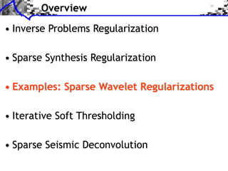
- 2. Overview • Inverse Problems Regularization • Sparse Synthesis Regularization • Examples: Sparse Wavelet Regularizations • Iterative Soft Thresholding • Sparse Seismic Deconvolution
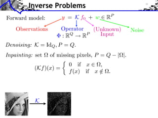
- 3. Inverse Problems Forward model: y = K f0 + w RP Observations Operator (Unknown) Noise : RQ RP Input
- 4. Inverse Problems Forward model: y = K f0 + w RP Observations Operator (Unknown) Noise : RQ RP Input Denoising: K = IdQ , P = Q.
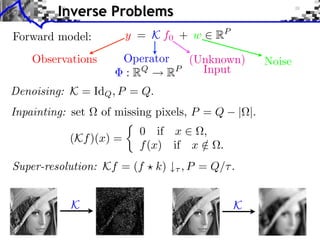
- 5. Inverse Problems Forward model: y = K f0 + w RP Observations Operator (Unknown) Noise : RQ RP Input Denoising: K = IdQ , P = Q. Inpainting: set of missing pixels, P = Q | |. 0 if x , (Kf )(x) = f (x) if x / . K
- 6. Inverse Problems Forward model: y = K f0 + w RP Observations Operator (Unknown) Noise : RQ RP Input Denoising: K = IdQ , P = Q. Inpainting: set of missing pixels, P = Q | |. 0 if x , (Kf )(x) = f (x) if x / . Super-resolution: Kf = (f k) , P = Q/ . K K
- 7. Inverse Problem in Medical Imaging Kf = (p k )1 k K
- 8. Inverse Problem in Medical Imaging Kf = (p k )1 k K Magnetic resonance imaging (MRI): ˆ Kf = (f ( )) ˆ f
- 9. Inverse Problem in Medical Imaging Kf = (p k )1 k K Magnetic resonance imaging (MRI): ˆ Kf = (f ( )) ˆ f Other examples: MEG, EEG, . . .
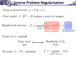
- 10. Inverse Problem Regularization Noisy measurements: y = Kf0 + w. Prior model: J : RQ R assigns a score to images.
- 11. Inverse Problem Regularization Noisy measurements: y = Kf0 + w. Prior model: J : RQ R assigns a score to images. 1 f argmin ||y Kf ||2 + J(f ) f RQ 2 Data fidelity Regularity
- 12. Inverse Problem Regularization Noisy measurements: y = Kf0 + w. Prior model: J : RQ R assigns a score to images. 1 f argmin ||y Kf ||2 + J(f ) f RQ 2 Data fidelity Regularity Choice of : tradeo Noise level Regularity of f0 ||w|| J(f0 )
- 13. Inverse Problem Regularization Noisy measurements: y = Kf0 + w. Prior model: J : RQ R assigns a score to images. 1 f argmin ||y Kf ||2 + J(f ) f RQ 2 Data fidelity Regularity Choice of : tradeo Noise level Regularity of f0 ||w|| J(f0 ) No noise: 0+ , minimize f argmin J(f ) f RQ ,Kf =y
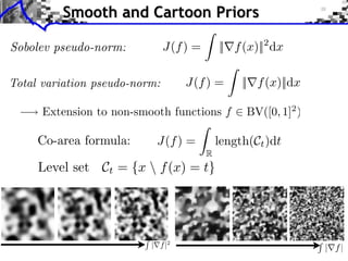
- 14. Smooth and Cartoon Priors J(f ) = || f (x)||2 dx | f |2
- 15. Smooth and Cartoon Priors J(f ) = || f (x)||2 dx J(f ) = || f (x)||dx J(f ) = length(Ct )dt R | f |2 | f|
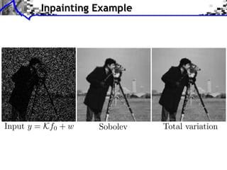
- 16. Inpainting Example Input y = Kf0 + w Sobolev Total variation
- 17. Overview • Inverse Problems Regularization • Sparse Synthesis Regularization • Examples: Sparse Wavelet Regularizations • Iterative Soft Thresholding • Sparse Seismic Deconvolution
- 18. Redundant Dictionaries Dictionary =( m )m RQ N ,N Q. Q N
- 19. Redundant Dictionaries Dictionary =( m )m RQ N ,N Q. Fourier: m = ei ·, m frequency Q N
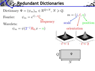
- 20. Redundant Dictionaries Dictionary =( m )m RQ N ,N Q. m = (j, , n) Fourier: m =e i ·, m frequency scale position Wavelets: m = (2 j R x n) orientation =1 =2 Q N
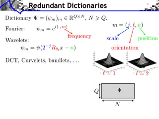
- 21. Redundant Dictionaries Dictionary =( m )m RQ N ,N Q. m = (j, , n) Fourier: m =e i ·, m frequency scale position Wavelets: m = (2 j R x n) orientation DCT, Curvelets, bandlets, . . . =1 =2 Q N
- 22. Redundant Dictionaries Dictionary =( m )m RQ N ,N Q. m = (j, , n) Fourier: m =e i ·, m frequency scale position Wavelets: m = (2 j R x n) orientation DCT, Curvelets, bandlets, . . . Synthesis: f = m xm m = x. =1 =2 Q =f x N Coe cients x Image f = x
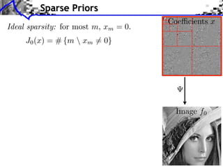
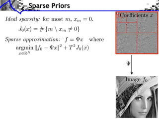
- 23. Sparse Priors Coe cients x Ideal sparsity: for most m, xm = 0. J0 (x) = # {m xm = 0} Image f0
- 24. Sparse Priors Coe cients x Ideal sparsity: for most m, xm = 0. J0 (x) = # {m xm = 0} Sparse approximation: f = x where argmin ||f0 x||2 + T 2 J0 (x) x2RN Image f0
- 25. Sparse Priors Coe cients x Ideal sparsity: for most m, xm = 0. J0 (x) = # {m xm = 0} Sparse approximation: f = x where argmin ||f0 x||2 + T 2 J0 (x) x2RN Orthogonal : = = IdN f0 , m if | f0 , m | > T, xm = 0 otherwise. ST Image f0 f= ST (f0 )
- 26. Sparse Priors Coe cients x Ideal sparsity: for most m, xm = 0. J0 (x) = # {m xm = 0} Sparse approximation: f = x where argmin ||f0 x||2 + T 2 J0 (x) x2RN Orthogonal : = = IdN f0 , m if | f0 , m | > T, xm = 0 otherwise. ST Image f0 f= ST (f0 ) Non-orthogonal : NP-hard.
- 27. Convex Relaxation: L1 Prior J0 (x) = # {m xm = 0} J0 (x) = 0 null image. Image with 2 pixels: J0 (x) = 1 sparse image. J0 (x) = 2 non-sparse image. x2 x1 q=0
- 28. Convex Relaxation: L1 Prior J0 (x) = # {m xm = 0} J0 (x) = 0 null image. Image with 2 pixels: J0 (x) = 1 sparse image. J0 (x) = 2 non-sparse image. x2 x1 q=0 q = 1/2 q=1 q = 3/2 q=2 q priors: Jq (x) = |xm |q (convex for q 1) m
- 29. Convex Relaxation: L1 Prior J0 (x) = # {m xm = 0} J0 (x) = 0 null image. Image with 2 pixels: J0 (x) = 1 sparse image. J0 (x) = 2 non-sparse image. x2 x1 q=0 q = 1/2 q=1 q = 3/2 q=2 q priors: Jq (x) = |xm |q (convex for q 1) m Sparse 1 prior: J1 (x) = |xm | m
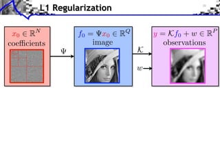
- 30. L1 Regularization x0 RN coe cients
- 31. L1 Regularization x0 RN f0 = x0 RQ coe cients image
- 32. L1 Regularization x0 RN f0 = x0 RQ y = Kf0 + w RP coe cients image observations K w
- 33. L1 Regularization x0 RN f0 = x0 RQ y = Kf0 + w RP coe cients image observations K w = K ⇥ ⇥ RP N
- 34. L1 Regularization x0 RN f0 = x0 RQ y = Kf0 + w RP coe cients image observations K w = K ⇥ ⇥ RP N Sparse recovery: f = x where x solves 1 min ||y x||2 + ||x||1 x RN 2 Fidelity Regularization
- 35. Noiseless Sparse Regularization Noiseless measurements: y = x0 x x= y x argmin |xm | x=y m
- 36. Noiseless Sparse Regularization Noiseless measurements: y = x0 x x x= x= y y x argmin |xm | x argmin |xm |2 x=y m x=y m
- 37. Noiseless Sparse Regularization Noiseless measurements: y = x0 x x x= x= y y x argmin |xm | x argmin |xm |2 x=y m x=y m Convex linear program. Interior points, cf. [Chen, Donoho, Saunders] “basis pursuit”. Douglas-Rachford splitting, see [Combettes, Pesquet].
- 38. Noisy Sparse Regularization Noisy measurements: y = x0 + w 1 x argmin ||y x||2 + ||x||1 x RQ 2 Data fidelity Regularization
- 39. Noisy Sparse Regularization Noisy measurements: y = x0 + w 1 x argmin ||y x||2 + ||x||1 x RQ 2 Equivalence Data fidelity Regularization x argmin ||x||1 || x y|| | x= x y|
- 40. Noisy Sparse Regularization Noisy measurements: y = x0 + w 1 x argmin ||y x||2 + ||x||1 x RQ 2 Equivalence Data fidelity Regularization x argmin ||x||1 || x y|| | x= Algorithms: x y| Iterative soft thresholding Forward-backward splitting see [Daubechies et al], [Pesquet et al], etc Nesterov multi-steps schemes.
- 41. Overview • Inverse Problems Regularization • Sparse Synthesis Regularization • Examples: Sparse Wavelet Regularizations • Iterative Soft Thresholding • Sparse Seismic Deconvolution
- 42. Image De-blurring Original f0 y = h f0 + w
- 43. Image De-blurring Original f0 y = h f0 + w Sobolev SNR=22.7dB Sobolev regularization: f = argmin ||f ⇥ h y||2 + ||⇥f ||2 f RN ˆ h(⇥) ˆ f (⇥) = y (⇥) ˆ ˆ |h(⇥)|2 + |⇥|2
- 44. Image De-blurring Original f0 y = h f0 + w Sobolev Sparsity SNR=22.7dB SNR=24.7dB Sobolev regularization: f = argmin ||f ⇥ h y||2 + ||⇥f ||2 f RN ˆ h(⇥) ˆ f (⇥) = y (⇥) ˆ ˆ |h(⇥)|2 + |⇥|2 Sparsity regularization: = translation invariant wavelets. 1 f = x where x argmin ||h ( x) y||2 + ||x||1 x 2
- 45. Comparison of Regularizations L2 regularization Sobolev regularization Sparsity regularization SNR SNR SNR opt opt opt L2 Sobolev Sparsity Invariant SNR=21.7dB SNR=22.7dB SNR=23.7dB SNR=24.7dB
- 46. Inpainting Problem K 0 if x , (Kf )(x) = f (x) if x / . Measures: y = Kf0 + w
- 47. Image Separation Model: f = f1 + f2 + w, (f1 , f2 ) components, w noise.
- 48. Image Separation Model: f = f1 + f2 + w, (f1 , f2 ) components, w noise.
- 49. Image Separation Model: f = f1 + f2 + w, (f1 , f2 ) components, w noise. Union dictionary: =[ 1, 2] RQ (N1 +N2 ) Recovered component: fi = i xi . 1 (x1 , x2 ) argmin ||f x||2 + ||x||1 x=(x1 ,x2 ) RN 2
- 52. Overview • Inverse Problems Regularization • Sparse Synthesis Regularization • Examples: Sparse Wavelet Regularizations • Iterative Soft Thresholding • Sparse Seismic Deconvolution
- 53. Sparse Regularization Denoising Denoising: y = x0 + w 2 RN , K = Id. ⇤ ⇤ Orthogonal-basis: = IdN , x = f. Regularization-based denoising: 1 x = argmin ||x y||2 + J(x) ? x2RN 2 P Sparse regularization: J(x) = m |xm |q (where |a|0 = (a))
- 54. Sparse Regularization Denoising Denoising: y = x0 + w 2 RN , K = Id. ⇤ ⇤ Orthogonal-basis: = IdN , x = f. Regularization-based denoising: 1 x = argmin ||x y||2 + J(x) ? x2RN 2 P Sparse regularization: J(x) = m |xm |q (where |a|0 = (a)) q x? m = ST (xm )
- 55. Surrogate Functionals Sparse regularization: ? 1 x 2 argmin E(x) = ||y x||2 + ||x||1 x2RN 2 ⇤ Surrogate functional: ⌧ < 1/|| || 1 2 1 E(x, x) = E(x) ˜ || (x x)|| + ||x ˜ x||2 ˜ 2 2⌧ E(·, x) ˜ E(·) x S ⌧ (u) x ˜
- 56. Surrogate Functionals Sparse regularization: ? 1 x 2 argmin E(x) = ||y x||2 + ||x||1 x2RN 2 ⇤ Surrogate functional: ⌧ < 1/|| || 1 2 1 E(x, x) = E(x) ˜ || (x x)|| + ||x ˜ x||2 ˜ 2 2⌧ E(·, x) ˜ Theorem: argmin E(x, x) = S ⌧ (u) ˜ E(·) x ⇤ where u = x ⌧ ( x x) ˜ x S ⌧ (u) x ˜ Proof: E(x, x) / 1 ||u ˜ 2 x||2 + ||x||1 + cst.
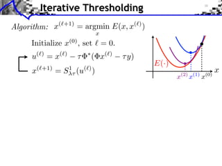
- 57. Iterative Thresholding Algorithm: x(`+1) = argmin E(x, x(`) ) x Initialize x(0) , set ` = 0. ⇤ u(`) = x(`) ⌧ ( x(`) ⌧ y) E(·) x(`+1) = S 1⌧ (u(`) ) (2) (1) (0) x x x x
- 58. Iterative Thresholding Algorithm: x(`+1) = argmin E(x, x(`) ) x Initialize x(0) , set ` = 0. ⇤ u(`) = x(`) ⌧ ( x(`) ⌧ y) E(·) x(`+1) = S 1⌧ (u(`) ) (2) (1) (0) x x x x Remark: x(`) 7! u(`) is a gradient descent of || x y||2 . 1 S`⌧ is the proximal step of associated to ||x||1 .
- 59. Iterative Thresholding Algorithm: x(`+1) = argmin E(x, x(`) ) x Initialize x(0) , set ` = 0. ⇤ u(`) = x(`) ⌧ ( x(`) ⌧ y) E(·) x(`+1) = S 1⌧ (u(`) ) (2) (1) (0) x x x x Remark: x(`) 7! u(`) is a gradient descent of || x y||2 . 1 S`⌧ is the proximal step of associated to ||x||1 . ⇤ Theorem: if ⌧ < 2/|| ||, then x(`) ! x? .
- 60. Overview • Inverse Problems Regularization • Sparse Synthesis Regularization • Examples: Sparse Wavelet Regularizations • Iterative Soft Thresholding • Sparse Seismic Deconvolution
- 61. Seismic Imaging
- 62. 1D Idealization Initial condition: “wavelet” = band pass filter h 1D propagation convolution f =h f h(x) f ˆ h( ) y = f0 h + w P
- 63. Pseudo Inverse Pseudo-inverse: ˆ+ ( ) = y ( ) f ˆ = f + = h+ ⇥ y = f0 + h+ ⇥ w h( ) ˆ ˆ where h+ ( ) = h( ) 1 ˆ ˆ Stabilization: h+ (⇥) = 0 if |h(⇥)| ˆ h( ) y = h f0 + w ˆ 1/h( ) f+
- 64. Sparse Spikes Deconvolution f with small ||f ||0 y=f h+w Sparsity basis: Diracs ⇥m [x] = [x m] 1 f = argmin ||f ⇥ h y||2 + |f [m]|. f RN 2 m
- 65. Sparse Spikes Deconvolution f with small ||f ||0 y=f h+w Sparsity basis: Diracs ⇥m [x] = [x m] 1 f = argmin ||f ⇥ h y||2 + |f [m]|. f RN 2 m Algorithm: < 2/|| ˆ || = 2/max |h(⇥)|2 ˜ • Inversion: f (k) = f (k) h ⇥ (h ⇥ f (k) y). ˜ f (k+1) [m] = S 1⇥ (f (k) [m])
- 66. Numerical Example f0 Choosing optimal : oracle, minimize ||f0 f || y=f h+w SNR(f0 , f ) f
- 67. Convergence Study Sparse deconvolution:f = argmin E(f ). f RN 1 Energy: E(f ) = ||h ⇥ f y||2 + |f [m]|. 2 m Not strictly convex = no convergence speed. log10 (E(f (k) )/E(f ) 1) log10 (||f (k) f ||/||f0 ||) k k
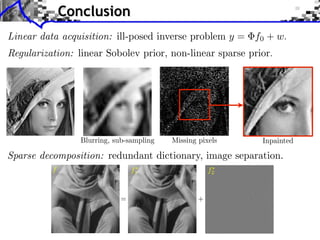
- 68. Conclusion
- 69. Conclusion
- 70. Conclusion